Tag Archives: Performance
Troubleshooting Calculation Performance Between Instances of Essbase
|
|||
|
|||
|
The purpose of this document is to provide information regarding Essbase calculation performance issues between two versions of Essbase or between two instances of Essbase on different platforms. Calculation performance differences between servers or Essbase versions can occur for many different reasons. These include differences in version, machine, outline design, and the amount of data. This document describes some items that can be checked and reviewed if you encounter any issues. |
|||
|
|
|||
|
To assist in locating an article of interest for future reference, consider adding a bookmark.
Once bookmarked the star will become yellow, and the article can be quickly accessed from the "Favorites" drop down menu. |
|||
|
|
|||
| |
System Metrics Collectors
The need to monitor and control the system performances is not new. What is new is the trend of clever, lightweight, easy to setup, open source metric collectors in the market, along with timeseries databases to store these metrics, and user friendly front ends through which to display and analyse the data.
In this post I will compare Telegraf, Collectl and Topbeat as lightweight metric collectors. All of them do a great job of collecting variety of useful system and application statistic data with minimal overhead to the servers. Each has the strength of easy configuration and accessible documentation but still there are some differences around range of input and outputs; how they extract the data, what metrics they collect and where they store them.
- Telegraf is part of the Influx TICK stack, and works with a vast variety of useful input plugins such as Elasticsearch, nginx, AWS and so on. It also supports a variety of outputs, obviously InfluxDB being the primary one. (Find out more…)
- Topbeat is a new tool from Elastic, the company behind Elasticsearch, Logstash, and Kibana. The Beats platform is evolving rapidly, and includes topbeat, winlogbeat, and packetbeat. In terms of metric collection its support for detailed metrics such as disk IO is relatively limited currently. (Find out more…)
- Collectl is a long-standing favourite of systems performance analysts, providing a rich source of data. This depth of complexity comes at a bit of a cost when it comes to the documentation’s accessibility, it being aimed firmly at a systems programmer! (Find out more…)
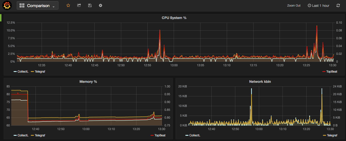
In this post I have used InfluxDB as the backend for storing the data, and Grafana as the front end visualisation tool. I will explain more about both tools later in this post.
In the screenshot below I have used Grafana dashboards to show “Used CPU”, “Used Memory” and “Network Traffic” stats from the mentioned collectors. As you can see the output of all three is almost the same. What makes them different is:
- What your infrastructure can support? For example, you cannot install Telegraf on old version of X Server.
- What input plugins do you need? The current version of Topbeat doesn’t support more detailed metrics such as disk IO and network stats.
- What storage do you want/need to use for the outputs? InfluxDB works as the best match for Telegraf data, whilst Beats pairs naturally with Elasticsearch
- What is your visualisation tool and what does it work with best. In all cases the best front end should natively support time series visualisations.

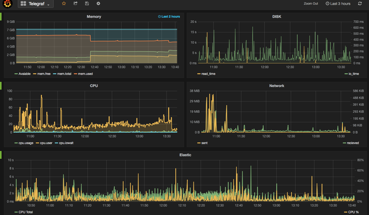
Next I am going to provide more details on how to download/install each of the mentioned metrics collector services, example commands are written for a linux system.
Telegraf
“An open source agent written in Go for collecting metrics and data on the system it’s running on or from other services. Telegraf writes data it collects to InfluxDB in the correct format.”
- Download and install InfluxDB:
sudo yum install -y https://s3.amazonaws.com/influxdb/influxdb-0.10.0-1.x86_64.rpm - Start the InfluxDB service:
sudo service influxdb start - Download Telegraf:
wget http://get.influxdb.org/telegraf/telegraf-0.12.0-1.x86_64.rpm - Install Telegraf:
sudo yum localinstall telegraf-0.12.0-1.x86_64.rpm - Start the Telegraf service:
sudo service telegraph start - Done!
The default configuration file for Telegraf sits in /etc/telegraf/telegraf.conf or a new config file can be generated using the -sample-config flag on the location of your choice: telegraf -sample-config > telegraf.conf . Update the config file to enable/disable/setup different input or outputs plugins e.g. I enabled network inputs: [[inputs.net]]. Finally to test the config files and to verify the output metrics run: telegraf -config telegraf.conf -test
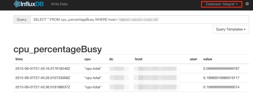
Once all ready and started, a new database called ‘telegraf’ will be added to the InfluxDB storage which you can connect and query. You will read more about InfluxDB in this post.
Collectl
Unlike most monitoring tools that either focus on a small set of statistics, format their output in only one way, run either interactively or as a daemon but not both, collectl tries to do it all. You can choose to monitor any of a broad set of subsystems which currently include buddyinfo, cpu, disk, inodes, infiniband, lustre, memory, network, nfs, processes, quadrics, slabs, sockets and tcp.
- Install collectl:
sudo yum install collectl - Update the Collectl config file at
/etc/collectl.confto turn on/off different switches and also to write the Collectl’s output logs to a database, i.e. InfluxDB - Restart Collectl service
sudo service collectl restart - Collectl will write its log in a new InfluxDB database called “graphite”.
Topbeat
Topbeat is a lightweight way to gather CPU, memory, and other per-process and system wide data, then ship it to (by default) Elasticsearch to analyze the results.
- Download Topbeat:
wget https://download.elastic.co/beats/topbeat/topbeat-1.2.1-x86_64.rpm - Install:
sudo yum local install topbeat-1.2.1-x86_64.rpm - Edit the topbeat.yml configuration file at
/etc/topbeatand set the output to elasticsearch or logstash. - If choosing elasticsearch as output, you need to load the index template, which lets Elasticsearch know which fields should be analyzed in which way. The recommended template file is installed by the Topbeat packages. You can either configure Topbeat to load the template automatically, Or you can run a shell script to load the template:
curl -XPUT 'http://localhost:9200/_template/topbeat -d@/etc/topbeat/topbeat.template.json - Run topbeat:
sudo /etc/init.d/topbeat start - To test your Topbeat Installation try:
curl -XGET 'http://localhost:9200/topbeat-*/_search?pretty' - TopBeat logs are written at
/var/log - Reference to output fields
Why write another metrics collector?
From everything that I have covered above, it is obvious that there is no shortage of open source agents for collecting metrics. Still you may come across a situation that none of the options could be used e.g. specific operating system (in this case, MacOS on XServe) that can’t support any of the options above. The below code is my version of light metric collector, to keep track of Disk IO stats, network, CPU and memory of the host where the simple bash script will be run.
The code will run through an indefinite loop until it is forced quit. Within the loop, first I have used a CURL request (InfluxDB API Reference) to create a database called OSStat, if the database name exists nothing will happen. Then I have used a variety of built-in OS tools to extract the data I needed. In my example sar -u for cpu, sar -n for network, vm_stat for memory, iotop for diskio could return the values I needed. With a quick search you will find many more options. I also used a combinations of awk, sed and grep to transform the values from these tools to the structure that I was easier to use on the front end. Finally I pushed the results to InfluxDB using the curl requests.
#!/bin/bash
export INFLUX_SERVER=$1
while [ 1 -eq 1 ];
do

#######CREATE DATABASE ########
curl -G http://$INFLUX_SERVER:8086/query  -s --data-urlencode "q=CREATE DATABASE OSStat" > /dev/null

####### CPU  #########
sar 1 1 -u | tail -n 1 | awk -v MYHOST=$(hostname)   '{  print "cpu,host="MYHOST"  %usr="$2",%nice="$3",%sys="$4",%idle="$5}' | curl -i -XPOST "http://${INFLUX_SERVER}:8086/write?db=OSStat"  -s --data-binary @- > /dev/null

####### Memory ##########
FREE_BLOCKS=$(vm_stat | grep free | awk '{ print $3 }' | sed 's/.//')
INACTIVE_BLOCKS=$(vm_stat | grep inactive | awk '{ print $3 }' | sed 's/.//')
SPECULATIVE_BLOCKS=$(vm_stat | grep speculative | awk '{ print $3 }' | sed 's/.//')
WIRED_BLOCKS=$(vm_stat | grep wired | awk '{ print $4 }' | sed 's/.//')

FREE=$((($FREE_BLOCKS+SPECULATIVE_BLOCKS)*4096/1048576))
INACTIVE=$(($INACTIVE_BLOCKS*4096/1048576))
TOTALFREE=$((($FREE+$INACTIVE)))
WIRED=$(($WIRED_BLOCKS*4096/1048576))
ACTIVE=$(((4096-($TOTALFREE+$WIRED))))
TOTAL=$((($INACTIVE+$WIRED+$ACTIVE)))

curl -i -XPOST "http://${INFLUX_SERVER}:8086/write?db=OSStat"  -s --data-binary  "memory,host="$(hostname)" Free="$FREE",Inactive="$INACTIVE",Total-free="$TOTALFREE",Wired="$WIRED",Active="$ACTIVE",total-used="$TOTAL > /dev/null

####### Disk IO ##########
iotop -t 1 1 -P | head -n 2  | grep 201 | awk -v MYHOST=$(hostname)
  '{ print "diskio,host="MYHOST" io_time="$6"read_bytes="$8*1024",write_bytes="$11*1024}'  | curl -i -XPOST "http://${INFLUX_SERVER}:8086/write?db=OSStat"  -s --data-binary @- > /dev/null

###### NETWORK ##########
sar -n DEV 1  |grep -v IFACE|grep -v Average|grep -v -E ^$ | awk -v MYHOST="$(hostname)" '{print "net,host="MYHOST",iface="$2" pktin_s="$3",bytesin_s="$4",pktout_s="$4",bytesout_s="$5}'|curl -i -XPOST "http://${INFLUX_SERVER}:8086/write?db=OSStat"  -s --data-binary @- > /dev/null

sleep 10;
done
InfluxDB Storage
“InfluxDB is a time series database built from the ground up to handle high write and query loads. It is the second piece of the TICK stack. InfluxDB is meant to be used as a backing store for any use case involving large amounts of timestamped data, including DevOps monitoring, application metrics, IoT sensor data, and real-time analytics.”
InfluxDB’s SQL-like query language is called InfluxQL, You can connect/query InfluxDB via Curl requests (mentioned above), command line or browser. The following sample InfluxQLs cover useful basic command line statements to get you started:
influx -- Connect to the database

SHOW DATABASES  -- Show existing databases, _internal is the embedded databased used for internal metrics

USE telegraf -- Make 'telegraf' the current database

SHOW MEASUREMENTS -- show all tables within current database

SHOW FIELD KEYS -- show tables definition within current database
InfluxDB also have a browser admin console that is by default accessible on port 8086. (Official Reference) (Read more on RittmanMead Blog)

Grafana Visualisation
“Grafana provides rich visualisation options best for working with time series data for Internet infrastructure and application performance analytics.”
Best to use InfluxDB as datasource for Grafana as Elasticsearch datasources doesn’t support all Grafana’s features e.g. functions behind the panels. Here is a good introduction video to visualisation with Grafana.
- Straight forward Installation:
sudo yum install -y https://grafanarel.s3.amazonaws.com/builds/grafana-2.6.0-1.x86_64.rpm - Start the service:
sudo service grafana-server start - Grafana is now ready to go on http://localhost:3000 (default username/password: admin/admin)

The post System Metrics Collectors appeared first on Rittman Mead Consulting.
System Metrics Collectors

The need to monitor and control the system performances is not new. What is new is the trend of clever, lightweight, easy to setup, open source metric collectors in the market, along with timeseries databases to store these metrics, and user friendly front ends through which to display and analyse the data.
In this post I will compare Telegraf, Collectl and Topbeat as lightweight metric collectors. All of them do a great job of collecting variety of useful system and application statistic data with minimal overhead to the servers. Each has the strength of easy configuration and accessible documentation but still there are some differences around range of input and outputs; how they extract the data, what metrics they collect and where they store them.
- Telegraf is part of the Influx TICK stack, and works with a vast variety of useful input plugins such as Elasticsearch, nginx, AWS and so on. It also supports a variety of outputs, obviously InfluxDB being the primary one. (Find out more...)
- Topbeat is a new tool from Elastic, the company behind Elasticsearch, Logstash, and Kibana. The Beats platform is evolving rapidly, and includes topbeat, winlogbeat, and packetbeat. In terms of metric collection its support for detailed metrics such as disk IO is relatively limited currently. (Find out more...)
- Collectl is a long-standing favourite of systems performance analysts, providing a rich source of data. This depth of complexity comes at a bit of a cost when it comes to the documentation’s accessibility, it being aimed firmly at a systems programmer! (Find out more...)
In this post I have used InfluxDB as the backend for storing the data, and Grafana as the front end visualisation tool. I will explain more about both tools later in this post.
In the screenshot below I have used Grafana dashboards to show "Used CPU", "Used Memory" and "Network Traffic" stats from the mentioned collectors. As you can see the output of all three is almost the same. What makes them different is:
- What your infrastructure can support? For example, you cannot install Telegraf on old version of X Server.
- What input plugins do you need? The current version of Topbeat doesn’t support more detailed metrics such as disk IO and network stats.
- What storage do you want/need to use for the outputs? InfluxDB works as the best match for Telegraf data, whilst Beats pairs naturally with Elasticsearch
- What is your visualisation tool and what does it work with best. In all cases the best front end should natively support time series visualisations.
Next I am going to provide more details on how to download/install each of the mentioned metrics collector services, example commands are written for a linux system.
Telegraf
"An open source agent written in Go for collecting metrics and data on the system it's running on or from other services. Telegraf writes data it collects to InfluxDB in the correct format."
- Download and install InfluxDB:
sudo yum install -y https://s3.amazonaws.com/influxdb/influxdb-0.10.0-1.x86_64.rpm - Start the InfluxDB service:
sudo service influxdb start - Download Telegraf:
wget http://get.influxdb.org/telegraf/telegraf-0.12.0-1.x86_64.rpm - Install Telegraf:
sudo yum localinstall telegraf-0.12.0-1.x86_64.rpm - Start the Telegraf service:
sudo service telegraph start - Done!
The default configuration file for Telegraf sits in /etc/telegraf/telegraf.conf or a new config file can be generated using the -sample-config flag on the location of your choice: telegraf -sample-config > telegraf.conf . Update the config file to enable/disable/setup different input or outputs plugins e.g. I enabled network inputs: [[inputs.net]]. Finally to test the config files and to verify the output metrics run: telegraf -config telegraf.conf -test
Once all ready and started, a new database called 'telegraf' will be added to the InfluxDB storage which you can connect and query. You will read more about InfluxDB in this post.
Collectl
Unlike most monitoring tools that either focus on a small set of statistics, format their output in only one way, run either interactively or as a daemon but not both, collectl tries to do it all. You can choose to monitor any of a broad set of subsystems which currently include buddyinfo, cpu, disk, inodes, infiniband, lustre, memory, network, nfs, processes, quadrics, slabs, sockets and tcp.
- Install collectl:
sudo yum install collectl - Update the Collectl config file at
/etc/collectl.confto turn on/off different switches and also to write the Collectl's output logs to a database, i.e. InfluxDB - Restart Collectl service
sudo service collectl restart - Collectl will write its log in a new InfluxDB database called “graphite”.
Topbeat
Topbeat is a lightweight way to gather CPU, memory, and other per-process and system wide data, then ship it to (by default) Elasticsearch to analyze the results.
- Download Topbeat:
wget https://download.elastic.co/beats/topbeat/topbeat-1.2.1-x86_64.rpm - Install:
sudo yum local install topbeat-1.2.1-x86_64.rpm - Edit the topbeat.yml configuration file at
/etc/topbeatand set the output to elasticsearch or logstash. - If choosing elasticsearch as output, you need to load the index template, which lets Elasticsearch know which fields should be analyzed in which way. The recommended template file is installed by the Topbeat packages. You can either configure Topbeat to load the template automatically, Or you can run a shell script to load the template:
curl -XPUT 'http://localhost:9200/_template/topbeat -d@/etc/topbeat/topbeat.template.json - Run topbeat:
sudo /etc/init.d/topbeat start - To test your Topbeat Installation try:
curl -XGET 'http://localhost:9200/topbeat-*/_search?pretty' - TopBeat logs are written at
/var/log - Reference to output fields
Why write another metrics collector?
From everything that I have covered above, it is obvious that there is no shortage of open source agents for collecting metrics. Still you may come across a situation that none of the options could be used e.g. specific operating system (in this case, MacOS on XServe) that can’t support any of the options above. The below code is my version of light metric collector, to keep track of Disk IO stats, network, CPU and memory of the host where the simple bash script will be run.
The code will run through an indefinite loop until it is forced quit. Within the loop, first I have used a CURL request (InfluxDB API Reference) to create a database called OSStat, if the database name exists nothing will happen. Then I have used a variety of built-in OS tools to extract the data I needed. In my example sar -u for cpu, sar -n for network, vm_stat for memory, iotop for diskio could return the values I needed. With a quick search you will find many more options. I also used a combinations of awk, sed and grep to transform the values from these tools to the structure that I was easier to use on the front end. Finally I pushed the results to InfluxDB using the curl requests.
#!/bin/bash
export INFLUX_SERVER=$1
while [ 1 -eq 1 ];
do

#######CREATE DATABASE ########
curl -G http://$INFLUX_SERVER:8086/query  -s --data-urlencode "q=CREATE DATABASE OSStat" > /dev/null

####### CPU  #########
sar 1 1 -u | tail -n 1 | awk -v MYHOST=$(hostname)   '{  print "cpu,host="MYHOST"  %usr="$2",%nice="$3",%sys="$4",%idle="$5}' | curl -i -XPOST "http://${INFLUX_SERVER}:8086/write?db=OSStat"  -s --data-binary @- > /dev/null

####### Memory ##########
FREE_BLOCKS=$(vm_stat | grep free | awk '{ print $3 }' | sed 's/.//')
INACTIVE_BLOCKS=$(vm_stat | grep inactive | awk '{ print $3 }' | sed 's/.//')
SPECULATIVE_BLOCKS=$(vm_stat | grep speculative | awk '{ print $3 }' | sed 's/.//')
WIRED_BLOCKS=$(vm_stat | grep wired | awk '{ print $4 }' | sed 's/.//')

FREE=$((($FREE_BLOCKS+SPECULATIVE_BLOCKS)*4096/1048576))
INACTIVE=$(($INACTIVE_BLOCKS*4096/1048576))
TOTALFREE=$((($FREE+$INACTIVE)))
WIRED=$(($WIRED_BLOCKS*4096/1048576))
ACTIVE=$(((4096-($TOTALFREE+$WIRED))))
TOTAL=$((($INACTIVE+$WIRED+$ACTIVE)))

curl -i -XPOST "http://${INFLUX_SERVER}:8086/write?db=OSStat"  -s --data-binary  "memory,host="$(hostname)" Free="$FREE",Inactive="$INACTIVE",Total-free="$TOTALFREE",Wired="$WIRED",Active="$ACTIVE",total-used="$TOTAL > /dev/null

####### Disk IO ##########
iotop -t 1 1 -P | head -n 2  | grep 201 | awk -v MYHOST=$(hostname)
  '{ print "diskio,host="MYHOST" io_time="$6"read_bytes="$8*1024",write_bytes="$11*1024}'  | curl -i -XPOST "http://${INFLUX_SERVER}:8086/write?db=OSStat"  -s --data-binary @- > /dev/null

###### NETWORK ##########
sar -n DEV 1  |grep -v IFACE|grep -v Average|grep -v -E ^$ | awk -v MYHOST="$(hostname)" '{print "net,host="MYHOST",iface="$2" pktin_s="$3",bytesin_s="$4",pktout_s="$4",bytesout_s="$5}'|curl -i -XPOST "http://${INFLUX_SERVER}:8086/write?db=OSStat"  -s --data-binary @- > /dev/null

sleep 10;
done
InfluxDB Storage
"InfluxDB is a time series database built from the ground up to handle high write and query loads. It is the second piece of the TICK stack. InfluxDB is meant to be used as a backing store for any use case involving large amounts of timestamped data, including DevOps monitoring, application metrics, IoT sensor data, and real-time analytics."
InfluxDB's SQL-like query language is called InfluxQL, You can connect/query InfluxDB via Curl requests (mentioned above), command line or browser. The following sample InfluxQLs cover useful basic command line statements to get you started:
influx -- Connect to the database

SHOW DATABASES  -- Show existing databases, _internal is the embedded databased used for internal metrics

USE telegraf -- Make 'telegraf' the current database

SHOW MEASUREMENTS -- show all tables within current database

SHOW FIELD KEYS -- show tables definition within current database
InfluxDB also have a browser admin console that is by default accessible on port 8086. (Official Reference) (Read more on RittmanMead Blog)
Grafana Visualisation
"Grafana provides rich visualisation options best for working with time series data for Internet infrastructure and application performance analytics."
Best to use InfluxDB as datasource for Grafana as Elasticsearch datasources doesn't support all Grafana's features e.g. functions behind the panels. Here is a good introduction video to visualisation with Grafana.
- Straight forward Installation:
sudo yum install -y https://grafanarel.s3.amazonaws.com/builds/grafana-2.6.0-1.x86_64.rpm - Start the service:
sudo service grafana-server start - Grafana is now ready to go on http://localhost:3000 (default username/password: admin/admin)
OBIEE 12c – Extended Subject Areas (XSA) and the Data Set Service

One of the big changes in OBIEE 12c for end users is the ability to upload their own data sets and start analysing them directly, without needing to go through the traditional data provisioning and modelling process and associated leadtimes. The implementation of this is one of the big architectural changes of OBIEE 12c, introducing the concept of the Extended Subject Areas (XSA), and the Data Set Service (DSS).
In this article we'll see some of how XSA and DSS work behind the scenes, providing an important insight for troubleshooting and performance analysis of this functionality.
What is an XSA?
An Extended Subject Area (XSA) is made up of a dataset, and associated XML data model. It can be used standalone, or "mashed up" in conjunction with a "traditional" subject area on a common field
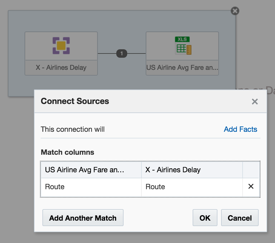
How is an XSA Created?
At the moment the following methods are available:
- "Add XSA" in Visual Analzyer, to upload an Excel (XLSX) document
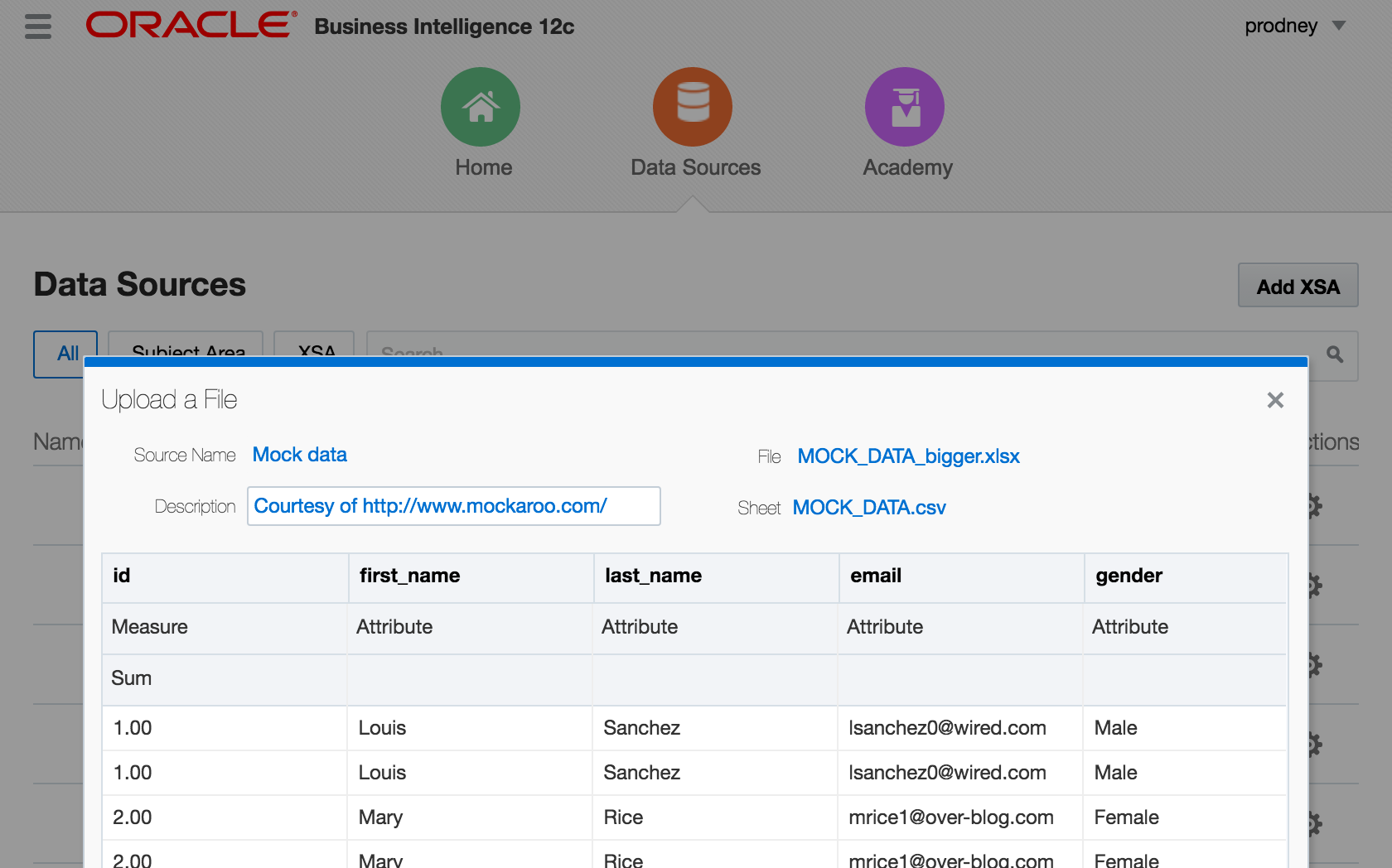
CREATE DATASETlogical SQL statement, that can be run through any interface to the BI Server, including 'Issue Raw SQL', nqcmd, JDBC calls, and so on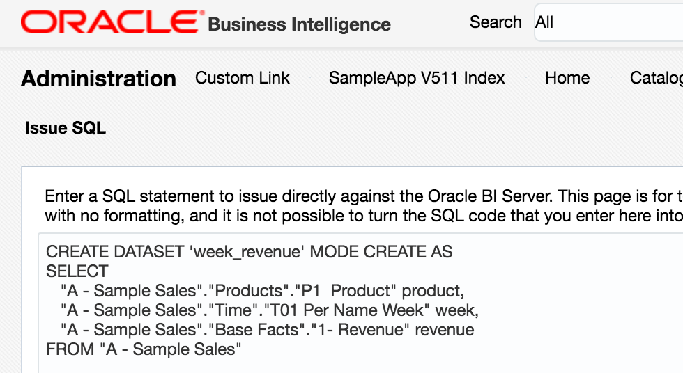
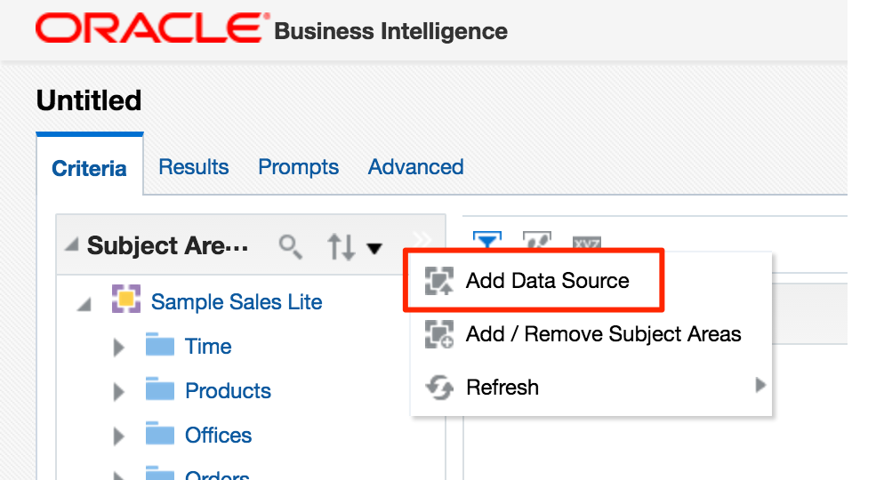
Add Data Source in Answers. Whilst this option shouldn't actually be present according to a this doc, it will be for any users of 12.2.1 who have uploaded the SampleAppLite BAR file so I'm including it here for completeness.
Under the covers, these all use the same REST API calls directly into datasetsvc. Note that these are entirely undocumented, and only for internal OBIEE component use. They are not intended nor supported for direct use.
How does an XSA work?
External Subject Areas (XSA) are managed by the Data Set Service (DSS). This is a java deployment (datasetsvc) running in the Managed Server (bi_server1), providing a RESTful API for the other OBIEE components that use it.
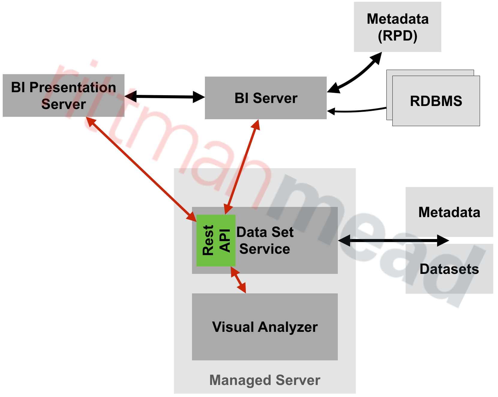
The end-user of the data, whether it's Visual Analyzer or the BI Server, send REST web service calls to DSS, storing and querying datasets within it.
Where is the XSA Stored?
By default, the data for XSA is stored on disk in SINGLETONDATADIRECTORY/components/DSS/storage/ssi, e.g. /app/oracle/biee/user_projects/domains/bi/bidata/components/DSS/storage/ssi
[oracle@demo ssi]$ ls -lrt /app/oracle/biee/user_projects/domains/bi/bidata/components/DSS/storage/ssi|tail -n5
-rw-r----- 1 oracle oinstall    8495 2015-12-02 18:01 7e43a80f-dcf6-4b31-b898-68616a68e7c4.dss
-rw-r----- 1 oracle oinstall  593662 2016-05-27 11:00 1beb5e40-a794-4aa9-8c1d-5a1c59888cb4.dss
-rw-r----- 1 oracle oinstall  131262 2016-05-27 11:12 53f59d34-2037-40f0-af21-45ac611f01d3.dss
-rw-r----- 1 oracle oinstall 1014459 2016-05-27 13:04 a4fc922d-ce0e-479f-97e4-1ddba074f5ac.dss
-rw-r----- 1 oracle oinstall 1014459 2016-05-27 13:06 c93aa2bd-857c-4651-bba2-a4f239115189.dss
They're stored using the format in which they were created, which is XLSX (via VA) or CSV (via CREATE DATASET)
[oracle@demo ssi]$ head 53f59d34-2037-40f0-af21-45ac611f01d3.dss
"7 Megapixel Digital Camera","2010 Week 27",44761.88
"MicroPod 60Gb","2010 Week 27",36460.0
"MP3 Speakers System","2010 Week 27",36988.86
"MPEG4 Camcorder","2010 Week 28",32409.78
"CompCell RX3","2010 Week 28",33005.91
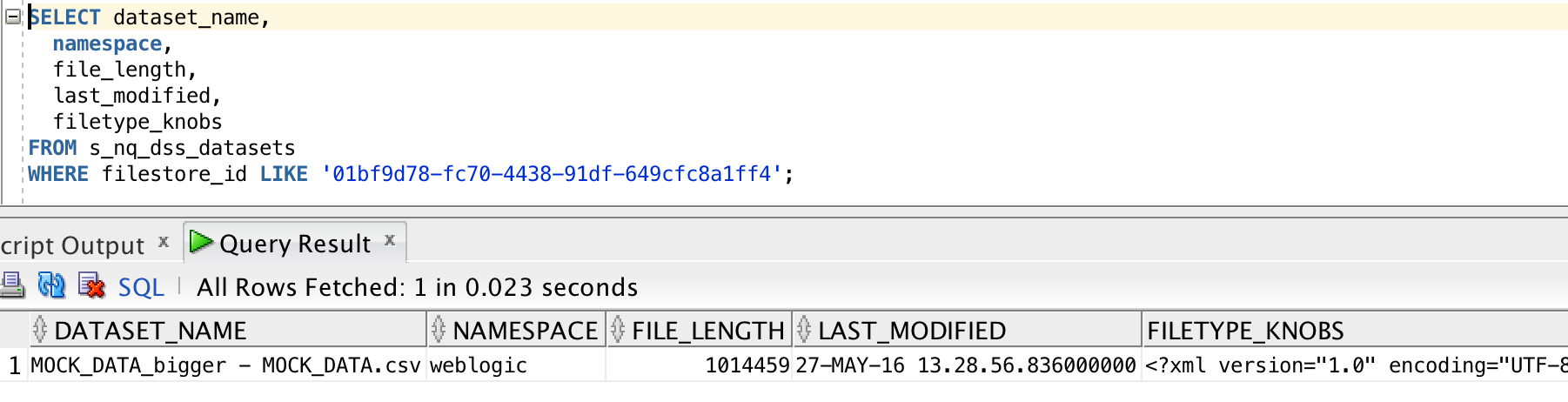
There's a set of DSS-related tables installed in the RCU schema BIPLATFORM, which hold information including the XML data model for the XSA, along with metadata such as the user that uploaded the file, when they uploaded, and then name of the file on disk:
How Can the Data Set Service be Configured?
The configuration file, with plenty of inline comments, is at ORACLEHOME/bi/endpointmanager/jeemap/dss/DSSREST_SERVICE.properties. From here you con update settings for the data set service including upload limits as detailed here.
XSA Performance
Since XSA are based on flat files stored in disk, we need to be very careful in their use. Whilst a database may hold billions of rows in a table with with appropriate indexing and partitioning be able to provide sub-second responses, a flat file can quickly become a serious performance bottleneck. Bear in mind that a flat file is just a bunch of data plopped on disk - there is no concept of indices, blocks, partitions -- all the good stuff that makes databases able to do responsive ad-hoc querying on selections of data.
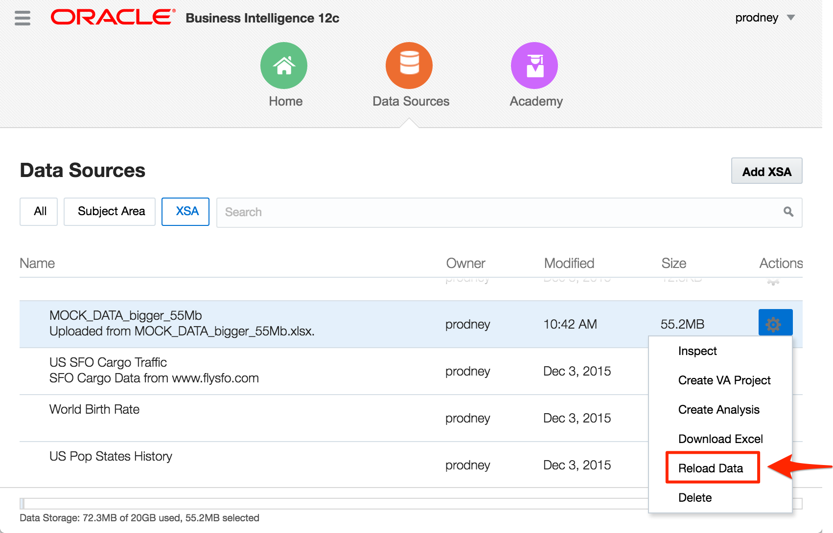
If you've got a 100MB Excel file with thousands of cells, and want to report on just a few of them, you might find it laggy - because whether you want to report on them on or not, at some point OBIEE is going to have to read all of them regardless. We can see how OBIEE is handling XSA under the covers by examining the query log. This used to be called nqquery.log in OBIEE 11g (and before), and in OBIEE 12c has been renamed obis1-query.log.
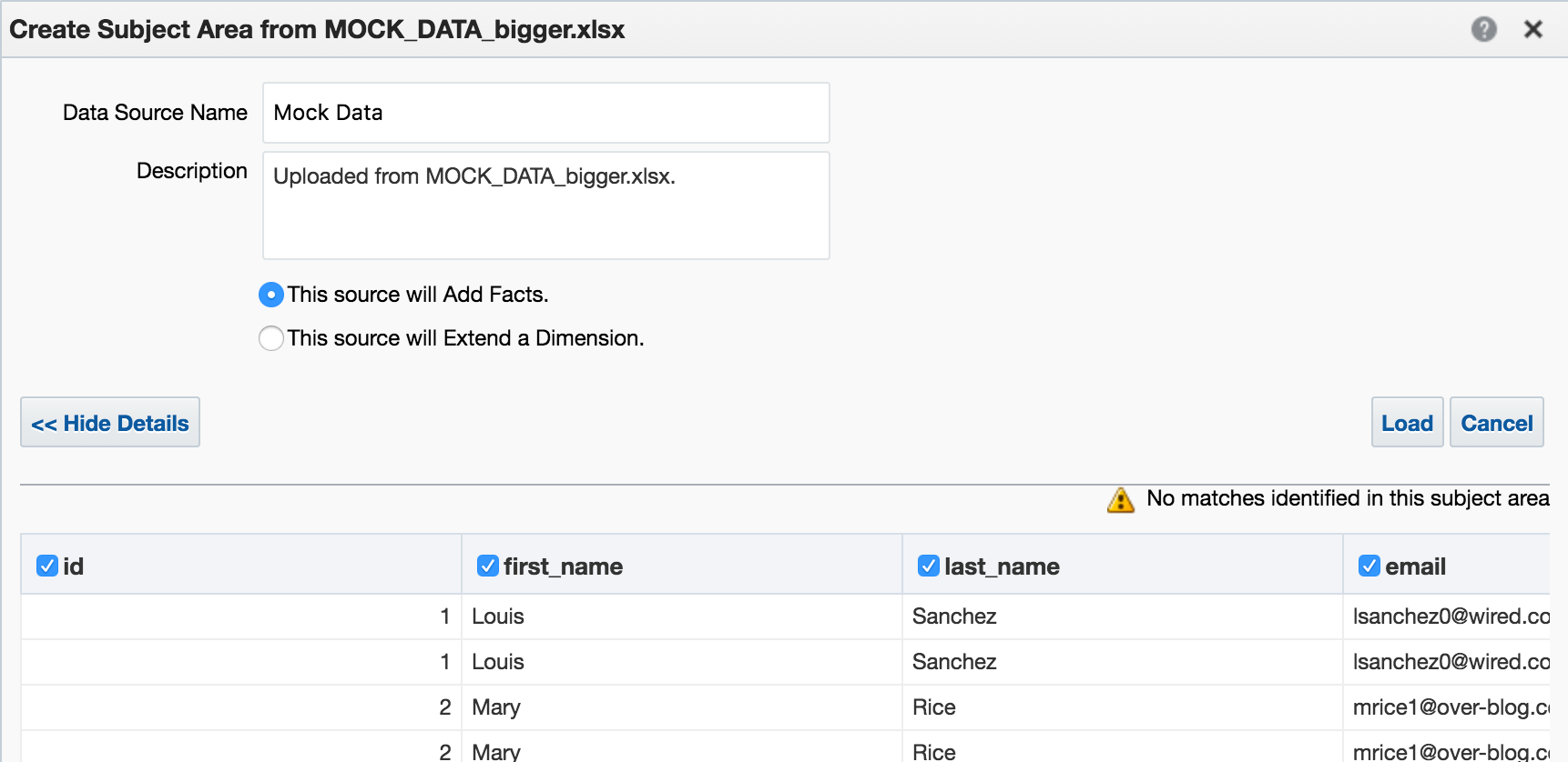
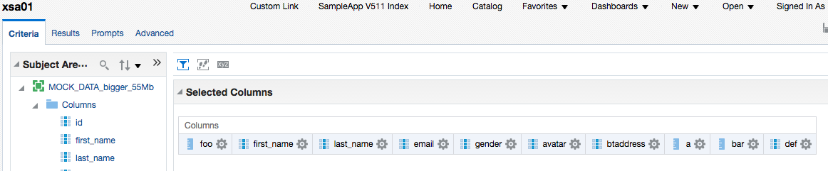
In this example here I'm using an Excel worksheet with 140,000 rows and 78 columns. Total filesize of the source XLSX on disk is ~55Mb.
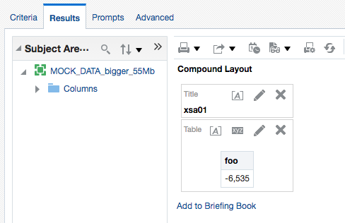
First up, I'll build a query in Answers with a couple of the columns:

The logical query uses the new XSA syntax:
SELECT
   0 s_0,
   XSA('prodney'.'MOCK_DATA_bigger_55Mb')."Columns"."first_name" s_1,
   XSA('prodney'.'MOCK_DATA_bigger_55Mb')."Columns"."foo" s_2
FROM XSA('prodney'.'MOCK_DATA_bigger_55Mb')
ORDER BY 2 ASC NULLS LAST
FETCH FIRST 5000001 ROWS ONLY
The query log shows
Rows 144000, bytes 13824000 retrieved from database query
Rows returned to Client 200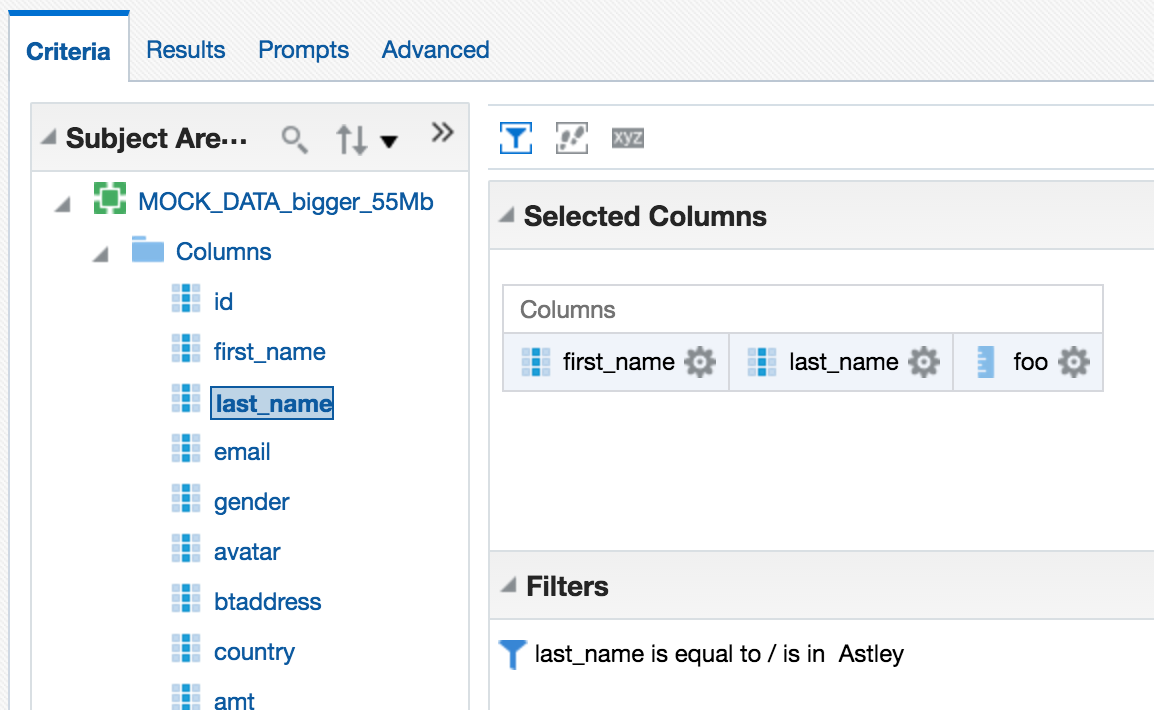 In the query log we can see that all the data has to come back from DSS to the BI Server, in order for it to filter it:
Rows 144000, bytes 23040000 retrieved from database
Physical query response time 24.195 (seconds),
Rows returned to Client 0
Note the time taken by DSS -- nearly 25 seconds. Compare this later on to when we see the XSA data served from a database, via the XSA Cache. In terms of BI Server (not XSA) caching, the query log shows that a cache entry was written for the above request:
Query Result Cache: [59124] The query for user 'prodney' was inserted into the query result cache. The filename is '/app/oracle/biee/user_projects/domains/bi/servers/obis1/cache/NQS__736113_56359_0.TBL'
 Unfortunately it didn't, and to return a single row of data required BI Server to fetch all the rows again - although looking at the byte count it appears it does prune the columns required since it's now just over 2Mb of data returned this time:
Rows 144000, bytes 2304000 retrieved from database
Rows returned to Client 1
Rows 144000, bytes 175104000
Rows returned to Client 1000
$ ls -l /app/oracle/biee/user_projects/domains/bi/servers/obis1/tmp/obis_temp
[...]
-rwxrwx--- 1 oracle oinstall 2910404 2016-06-01 14:08 nQS_AG_22345_7503_7c9c000a_50906091.TMP
-rwxrwx--- 1 oracle oinstall   43476 2016-06-01 14:08 nQS_AG_22345_7504_7c9c000a_50906091.TMP
-rw------- 1 oracle oinstall 6912000 2016-06-01 14:08 nQS_AG_22345_7508_7c9c000a_50921949.TMP
-rw------- 1 oracle oinstall  631375 2016-06-01 14:08 nQS_EX_22345_7506_7c9c000a_50921652.TMP
-rw------- 1 oracle oinstall 3670016 2016-06-01 14:08 nQS_EX_22345_7507_7c9c000a_50921673.TMP
[...]
You can read more about BI Server's use of temporary files and the impact that it can have on system performance and particularly I/O bandwidth in this OTN article here.
So - as the expression goes - "buyer beware". XSA is an excellent feature, but used in its default configuration with files stored on disk it has the potential to wreak havoc if abused.
XSA Caching
If you're planning to use XSA seriously, you should set up the database-based XSA Cache. This is described in detail in the PDF document attached to My Oracle Support note OBIEE 12c: How To Configure The External Subject Area (XSA) Cache For Data Blending| Mashup And Performance (Doc ID 2087801.1).
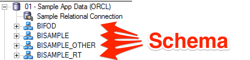
In a proper implementation you would follow in full the document, including provisioning a dedicated schema and tablespace for holding the data (to make it easier to manage and segregate from other data), but here I'm just going to use the existing RCU schema (BIPLATFORM), along with the Physical mapping already in the RPD (10 - System DB (ORCL)):
In NQSConfig.INI, under the XSA_CACHE section, I set:
ENABLE = YES;

# The schema and connection pool where the XSA data will be cached.
PHYSICAL_SCHEMA = "10 - System DB (ORCL)"."Catalog"."dbo";
CONNECTION_POOL = "10 - System DB (ORCL)"."UT Connection Pool";
/app/oracle/biee/user_projects/domains/bi/bitools/bin/stop.sh -i obis1 && /app/oracle/biee/user_projects/domains/bi/bitools/bin/start.sh -i obis1
Per the document, note that in the BI Server log there's an entry indicating that the cache has been successfully started:
[101001] External Subject Area cache is started successfully using configuration from the repository with the logical name ssi.
[101017] External Subject Area cache has been initialized. Total number of entries: 0 Used space: 0 bytes Maximum space: 107374182400 bytes Remaining space: 107374182400 bytes. Cache table name prefix is XC2875559987.
-- Sending query to database named 10 - System DB (ORCL) (id: <<79879>> XSACache Create table Gateway), connection pool named UT Connection Pool, logical request hash b4de812e, physical request hash 5847f2ef:
CREATE TABLE dbo.XC2875559987_ZPRODNE1926129021 ( id3209243024 DOUBLE PRECISION, first_n[..]
Or rather, it doesn't, because PHYSICALSCHEMA seems to want the literal physical schema, rather than the logical physical one (?!) that the USAGETRACKING configuration stanza is happy with in referencing the table.
Properties: description=<<79879>> XSACache Create table Exchange; producerID=0x1561aff8; requestID=0xfffe0034; sessionID=0xfffe0000; userName=prodney;
[nQSError: 17001] Oracle Error code: 1918, message: ORA-01918: user 'DBO' does not exist
I'm trying to piggyback on SA511's existing configruation, which uses catalog.schema notation:

Instead of the more conventional approach to have the actual physical schema (often used in conjunction with 'Require fully qualified table names' in the connection pool):
So now I'll do it properly, and create a database and schema for the XSA cache - I'm still going to use the BIPLATFORM schema though...
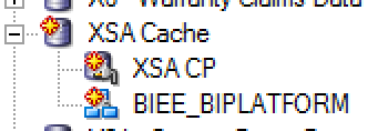
Updated NQSConfig.INI:
[ XSA_CACHE ]

ENABLE = YES;

# The schema and connection pool where the XSA data will be cached.
PHYSICAL_SCHEMA = "XSA Cache"."BIEE_BIPLATFORM";
CONNECTION_POOL = "XSA Cache"."XSA CP";
-- Sending query to database named XSA Cache (id: <<65685>> XSACache Create table Gateway), connection pool named XSA CP, logical request hash 9a548c60, physical request hash ccc0a410: [[
CREATE TABLE BIEE_BIPLATFORM.XC2875559987_ZPRODNE1645894381 ( id3209243024 DOUBLE PRECISION, first_name2360035083 VARCHAR2(17 CHAR), [...]
as well as a stats gather:
-- Sending query to database named XSA Cache (id: <<65685>> XSACache Collect statistics Gateway), connection pool named XSA CP, logical request hash 9a548c60, physical request hash d73151bb:
BEGIN DBMS_STATS.GATHER_TABLE_STATS(ownname => 'BIEE_BIPLATFORM', tabname => 'XC2875559987_ZPRODNE1645894381' , estimate_percent => 5 , method_opt => 'FOR ALL COLUMNS SIZE AUTO' ); END;
Although I do note that it is used a fixed estimatepercent instead of the recommended AUTOSAMPLE_SIZE. The table itself is created with a fixed prefix (as specified in the obis1-diagnostic.log at initialisation), and holds a full copy of the XSA (not just the columns in the query that triggered the cache creation):
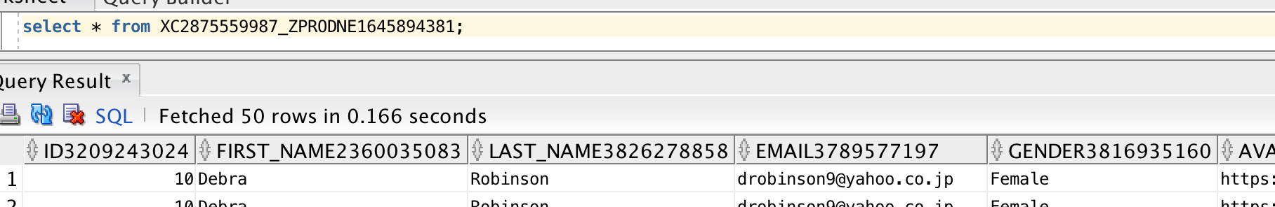
With the dataset cached, the query is then run and the query log shows a XSA cache hit
External Subject Area cache hit for 'prodney'.'MOCK_DATA_bigger_55Mb'/Columns :
Cache entry shared_cache_key = 'prodney'.'MOCK_DATA_bigger_55Mb',
table name = BIEE_BIPLATFORM.XC2875559987_ZPRODNE2128899357,
row count = 144000,
entry size = 201326592 bytes,
creation time = 2016-06-01 20:14:26.829,
creation elapsed time = 49779 ms,
descriptor ID = /app/oracle/biee/user_projects/domains/bi/servers/obis1/xsacache/NQSXSA_BIEE_BIPLATFORM.XC2875559987_ZPRODNE2128899357_2.CACHE
with the resulting physical query fired at the XSA cache table (replacing what would have gone against the DSS web service):
-- Sending query to database named XSA Cache (id: <<65357>>), connection pool named XSA CP, logical request hash 9a548c60, physical request hash d3ed281d: [[
WITH
SAWITH0 AS (select T1000001.first_name2360035083 as c1,
     T1000001.last_name3826278858 as c2,
     sum(T1000001.foo2363149668) as c3
from
     BIEE_BIPLATFORM.XC2875559987_ZPRODNE1645894381 T1000001
group by T1000001.first_name2360035083, T1000001.last_name3826278858)
select D1.c1 as c1, D1.c2 as c2, D1.c3 as c3, D1.c4 as c4 from ( select 0 as c1,
     D102.c1 as c2,
     D102.c2 as c3,
     D102.c3 as c4
from
     SAWITH0 D102
order by c2, c3 ) D1 where rownum <= 5000001
It's important to point out the difference of what's happening here: the aggregation has been pushed down to the database, meaning that the BI Server doesn't have to. In performance terms, this is a Very Good Thing usually.
Rows 988, bytes 165984 retrieved from database query
Rows returned to Client 988
 The BI Server does pick this up and repopulates the XSA Cache.
The XSA cache entry itself is 192Mb in size - generated from a 55Mb upload file. The difference will be down to data types and storage methods etc. However, that it is larger in the XSA Cache (database) than held natively (flat file) doesn't really matter, particularly if the data is being aggregated and/or filtered, since the performance benefit of pushing this work to the database will outweigh the overhead of storage space. Consider this example here, where I run an analysis pulling back 44 columns (of the 78 in the spreadsheet) and hit the XSA cache, it runs in just over a second, and transfers from the database a total of 5.3Mb (the data is repeated, so rolls up):
The BI Server does pick this up and repopulates the XSA Cache.
The XSA cache entry itself is 192Mb in size - generated from a 55Mb upload file. The difference will be down to data types and storage methods etc. However, that it is larger in the XSA Cache (database) than held natively (flat file) doesn't really matter, particularly if the data is being aggregated and/or filtered, since the performance benefit of pushing this work to the database will outweigh the overhead of storage space. Consider this example here, where I run an analysis pulling back 44 columns (of the 78 in the spreadsheet) and hit the XSA cache, it runs in just over a second, and transfers from the database a total of 5.3Mb (the data is repeated, so rolls up):
Rows 1000, bytes 5576000 retrieved from database
Rows returned to Client 1000
Rows 144000, bytes 801792000 Retrieved from database
Physical query response time 22.086 (seconds)
Rows returned to Client 1000
$  ls -l /app/oracle/biee/user_projects/domains/bi/servers/obis1/tmp/obis_temp
[...]]
-rwxrwx--- 1 oracle oinstall 10726190 2016-06-01 21:04 nQS_AG_29733_261_ebd70002_75835908.TMP
-rwxrwx--- 1 oracle oinstall   153388 2016-06-01 21:04 nQS_AG_29733_262_ebd70002_75835908.TMP
-rw------- 1 oracle oinstall 24192000 2016-06-01 21:04 nQS_AG_29733_266_ebd70002_75862509.TMP
-rw------- 1 oracle oinstall  4195609 2016-06-01 21:04 nQS_EX_29733_264_ebd70002_75861716.TMP
-rw------- 1 oracle oinstall 21430272 2016-06-01 21:04 nQS_EX_29733_265_ebd70002_75861739.TMP
As a reminder - this isn't "Bad", it's just not optimal (response time of 50 seconds vs 1 second), and if you scale that kind of behaviour by many users with many datasets, things could definitely get hairy for all users of the system. Hence - use the XSA Cache.
As a final point, with the XSA Cache being in the database the standard range of performance optimisations are open to us - indexing being the obvious one. No indexes are built against the XSA Cache table by default, which is fair enough since OBIEE has no idea what the key columns on the data are, and the point of mashups is less to model and optimise the data but to just get it up there in front of the user. So you could index the table if you knew the key columns that were going to be filtered against, or you could even put it into memory (assuming you've licensed the option).
The MoS document referenced above also includes further performance recommendations for XSA, including the use of RAM Disk for XSA cache metadata files, as well as the managed server temp folder
Summary
External Subject Areas are great functionality, but be aware of the performance implications of not being able to push down common operations such as filtering and aggregation. Set up XSA Caching if you are going to be using XSA properly.
If you're interested in the direction of XSA and the associated Data Set Service, this slide deck from Oracle's Socs Cappas provides some interesting reading. Uploading Excel files into OBIEE looks like just the beginning of what the Data Set Service is going to enable!
New OTN Article – OBIEE Performance Analytics : Analysing the Impact of Suboptimal Design
I’m pleased to have recently had my first article published on the Oracle Technology Network (OTN). You can read it in its full splendour and glory (!) over there, but I thought I’d give a bit of background to it here and the tools demonstrated within.
OBIEE Performance Analytics Dashboards
One of the things that we frequently help our clients with is reviewing and optimising the performance of their OBIEE systems. As part of this we’ve built up a wealth of experience in the kind of suboptimal design patterns that can cause performance issues, as well as how to go about identifying them empirically. Getting a full stack view on OBIEE performance behaviour is key to demonstrating where an issue lies, prior to being able to resolve it and proving it fixed, and for this we use the Rittman Mead OBIEE Performance Analytics Dashboards.

A common performance issue that we see is analyses and/or RPDs built in such a way that the BI Server inadvertently returns many gigabytes of data from the database and in doing so often has to dump out to disk whilst processing it. This can create large NQS_tmp files, impacting the disk space available (sometimes critically), and the disk I/O subsystem. This is the basis of the OTN article that I wrote, and you can read the full article on OTN to find out more about how this can be a problem and how to go about resolving it.
OBIEE implementations that cause heavy use of temporary files on disk by the BI Server can result in performance problems. Until recently in OBIEE it was really difficult to track because of the transitory nature of the files. By the time the problem had been observed (for example, disk full messages), the query responsible had moved on and so the temporarily files deleted. At Rittman Mead we have developed lightweight diagnostic tools that collect, amongst other things, the amount of temporary disk space used by each of the OBIEE components.

This can then be displayed as part of our Performance Analytics Dashboards, and analysed alongside other performance data on the system such as which queries were running, disk I/O rates, and more:

Because the Performance Analytics Dashboards are built in a modular fashion it is easy to customise them to suit specific analysis requirements. In this next example you can see performance data from Oracle being analysed by OBIEE dashboard page in order to identify the cause of poorly-performing reports:

We’ve put online a set of videos here demonstrating the Performance Analytics Dashboards, and explaining in each case how they can help you quickly and accurately diagnose OBIEE performance problems.
You can read more about our Performance Analytics offering here, or get in touch to find out more!
The post New OTN Article – OBIEE Performance Analytics : Analysing the Impact of Suboptimal Design appeared first on Rittman Mead Consulting.