Tag Archives: Big Data
Stream Analytics and Processing with Kafka and Oracle Stream Analytics
In my previous post I looked the latest release of Oracle Stream Analytics (OSA), and saw how it provided a graphical interface to "Fast Data". Users can analyse streaming data as it arrives based on conditions and rules. They can also transform the stream data, publishing it back out as a stream in its own right. In this article we'll see how OSA can be used with Kafka.
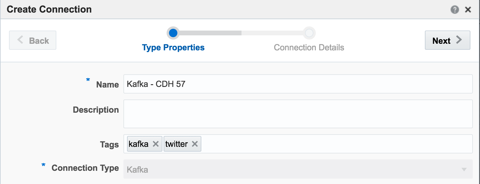
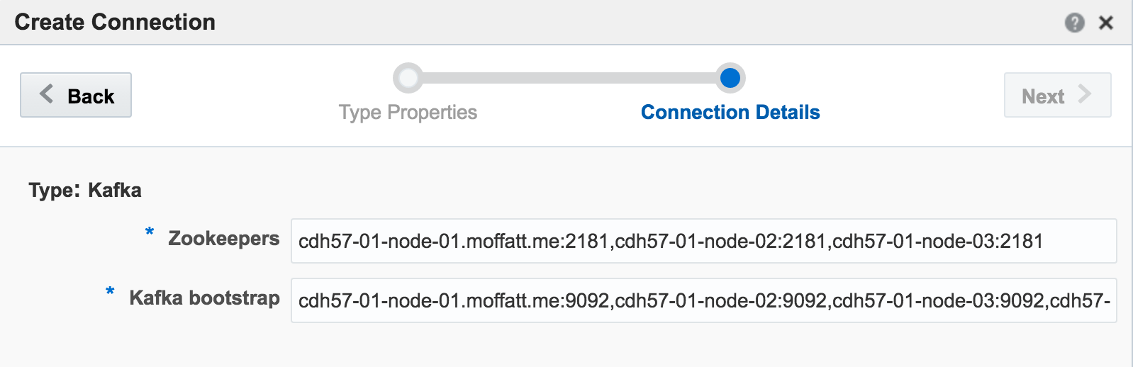
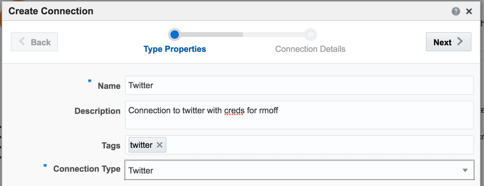
Kafka is one of the foremost streaming technologies nowadays, for very good reasons. It is highly scalable and flexible, supporting multiple concurrent consumers. Oracle Streaming Analytics supports Kafka as both a source and target. To set up an inbound stream from Kafka, first we define the Connection:
 If you get an error at this point of
 Unable to deploy OEP application then check the OSA log - it could be a connectivity issue to Zookeeper.
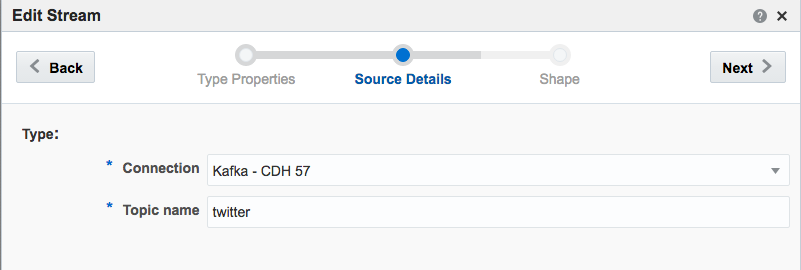
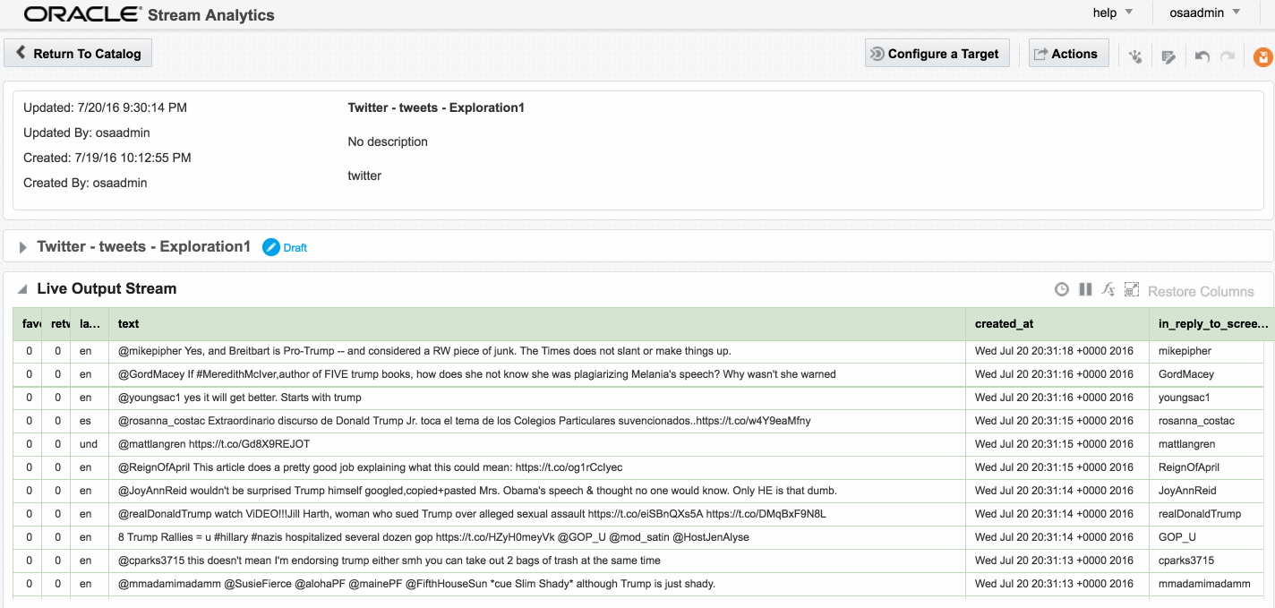
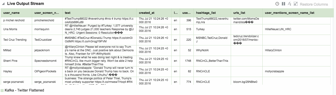
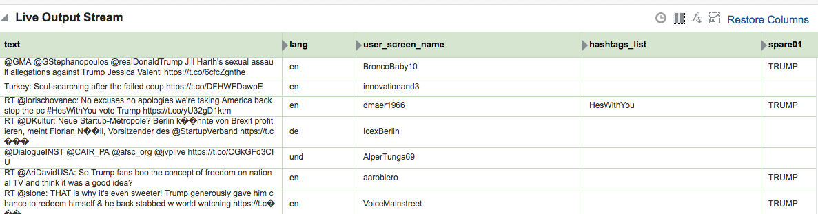
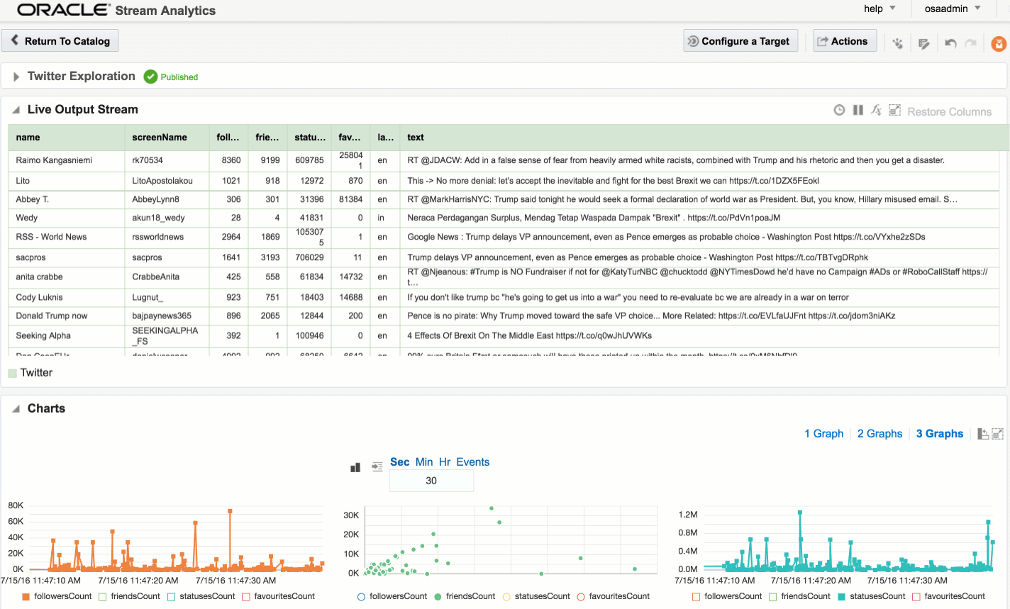
Exception in thread "SpringOsgiExtenderThread-286" org.springframework.beans.FatalBeanException:
Error in context lifecycle initialization; nested exception is com.bea.wlevs.ede.api.EventProcessingException:
org.I0Itec.zkclient.exception.ZkTimeoutException:
Unable to connect to zookeeper server within timeout: 6000
Assuming that the Stream is saved with no errors, you can then create an Exploration based on the stream and all being well, the live tweets are soon shown. Unlike the example at the top of this article, these tweets are coming in via Kafka, rather than the built-in OSA Twitter Stream. This is partly to demonstrate the Kafka capabilities, but also because the built-in OSA Twitter Stream only includes a subset of the available twitter data fields.
Avro? Nope.
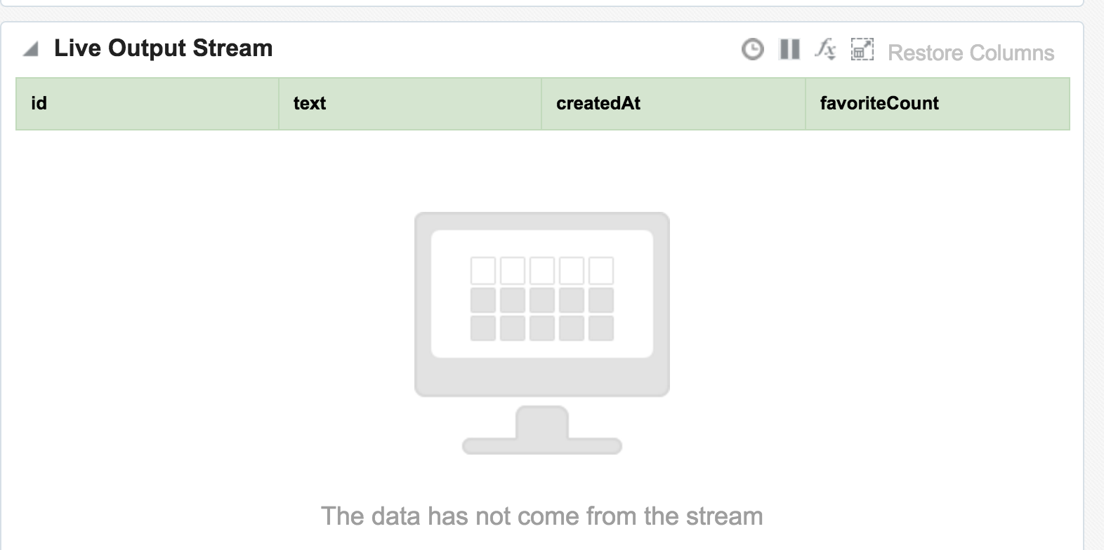
Data in Kafka can be serialised in many formats, including Avro - which OSA doesn’t seem to like. No error is thrown to the GUI but the exploration remains blank.
line 1:0 no viable alternative at character '?'
line 1:1 no viable alternative at character '?'
line 1:2 no viable alternative at character '?'
line 1:3 no viable alternative at character '?'
line 1:4 no viable alternative at character '?'
line 1:5 no viable alternative at character '?'
line 1:6 no viable alternative at character '?'
line 1:7 no viable alternative at character '?'
line 1:8 no viable alternative at character ''
JSON? Kinda.
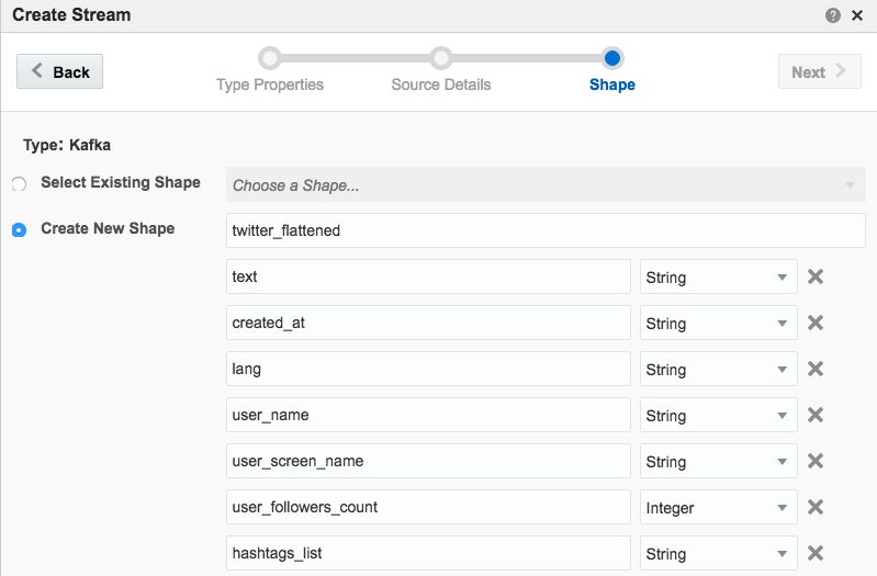
One of the challenges that I found working with OSA was defining the “Shape” (data model) of the inbound stream data. JSON is a format used widely as a technology-agnostic data interchange format, including for the twitter data that I was working with. You can see a sample record here. One of the powerful features of JSON is its ability to nest objects in a record, as well as create arrays of them. You can read more about this detail in a recent article I wrote here. Unfortunately it seems that OSA does not support flattening out JSON, meaning that only elements in the root of the model are accessible. For twitter, that means we can see the text, and who it was in reply to, but not the user who tweeted it, since the latter is a nested element (along with many other fields, including hashtags which are also an array):root
|-- created_at: string (nullable = true)
|-- entities: struct (nullable = true)
| |-- hashtags: array (nullable = true)
| | |-- element: struct (containsNull = true)
| | | |-- indices: array (nullable = true)
| | | | |-- element: long (containsNull = true)
| | | |-- text: string (nullable = true)
| |-- user_mentions: array (nullable = true)
| | |-- element: struct (containsNull = true)
| | | |-- id: long (nullable = true)
| | | |-- id_str: string (nullable = true)
| | | |-- indices: array (nullable = true)
| | | | |-- element: long (containsNull = true)
| | | |-- name: string (nullable = true)
| | | |-- screen_name: string (nullable = true)
|-- source: string (nullable = true)
|-- text: string (nullable = true)
|-- timestamp_ms: string (nullable = true)
|-- truncated: boolean (nullable = true)
|-- user: struct (nullable = true)
| |-- followers_count: long (nullable = true)
| |-- following: string (nullable = true)
| |-- friends_count: long (nullable = true)
| |-- name: string (nullable = true)
| |-- screen_name: string (nullable = true)mutate to bring nested objects up to the root level. Sample code:
mutate {
    add_field => { "user_name" => "%{[user][name]}" }
    add_field => { "user_screen_name" => "%{[user][screen_name]}" }
}
ruby {
    code => 'event["hashtags_array"] = event["[entities][hashtags]"].collect { |m| m["text"] } unless event["[entities][hashtags]"].nil?
             event["hashtags_list"] = event["hashtags_array"].join(",")  unless event["[hashtags_array]"].nil?'
}
You can find the full Logstash code on gist here. With this logstash code running I set up a new OSA Stream pointing to the new Kafka topic that Logstash was writing, and added the flattened fields to the Shape:
Other Shape Gotchas
One of the fields in Twitter data is ‘source’ - which unfortunately is a reserved identifier in the CQL language that OSA uses behind the scenes.
Caused By: org.springframework.beans.FatalBeanException: Exception initializing channel; nested exception is com.bea.wlevs.ede.api.ConfigurationException: Event type [sx-10-16-Kafka_Technology_Tweets_JSON-1] of channel [channel] uses invalid or reserved CQL identifier = , sourceIt’s not clear how to define a shape in which the source data field is named after a reserved identifier.
Further Exploration of Twitter Streams with OSA
Using the flattened Twitter stream coming via Kafka that I demonstrated above, let’s now look at more OSA functionality.
Depending on the source of your data stream, and your purpose for analysing it, you may well want to filter out certain content. This can be done from the Exploration screen:

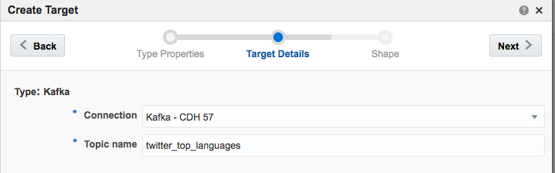
Kafka Stream Transformation with OSA
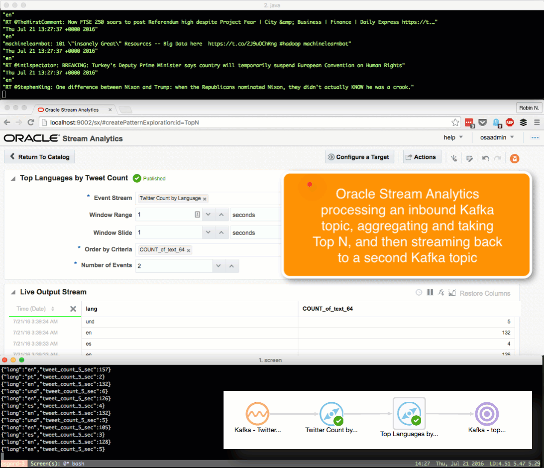
Here we’ll see how OSA can be used to ingest one Kafka topic, apply a transformation, and stream it to another Kafka topic.
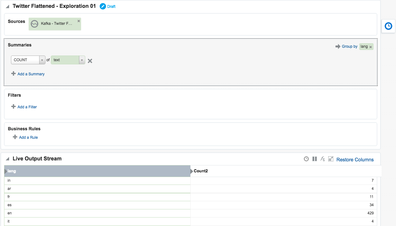
The OSA exploration screen offers a basic aggregation (‘summary’) function, here showing the number of tweets per language:
Taking the summarised stream (count of tweets, by language) I first Publish the exploration, making it available for use as the input to a subsequent exploration. Then from the Catalog page select a Pattern, which I’m going to use to build a stream showing the most common languages in the past five seconds. With the Top N pattern you specify the event stream (in this case, the summarised stream that I built above), and the metric by which to order the events which here is the count of tweets per language.
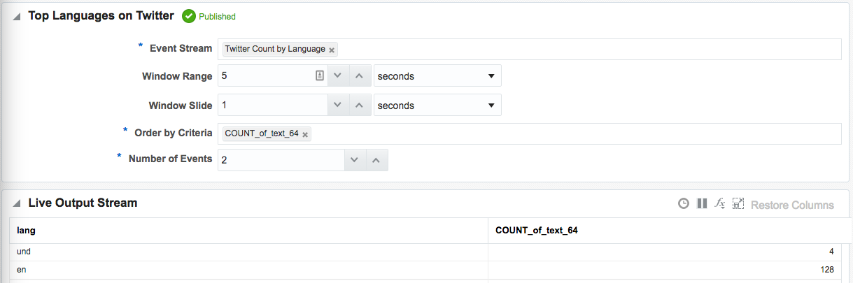
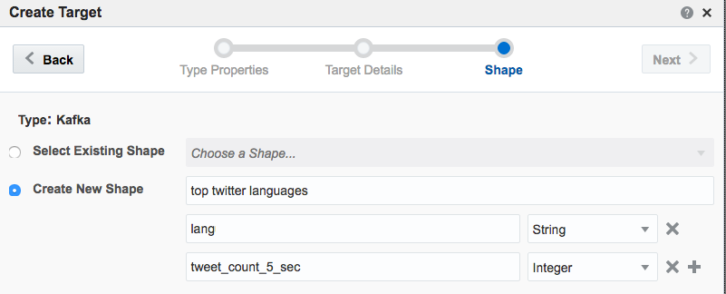
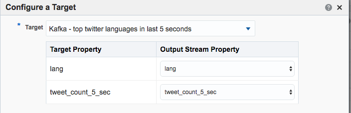
Note that I’ve defined a new Shape here based on the columns in the pattern. In the pattern itself I renamed the COUNT column to a clearer one (tweetcount5_sec). Renaming it wasn’t strictly necessary since it’s possible to define the field/shape mapping when you configure the Target:
kafka-console-consumer can see the topic being populated in realtime by OSA:
OSA and Spatial
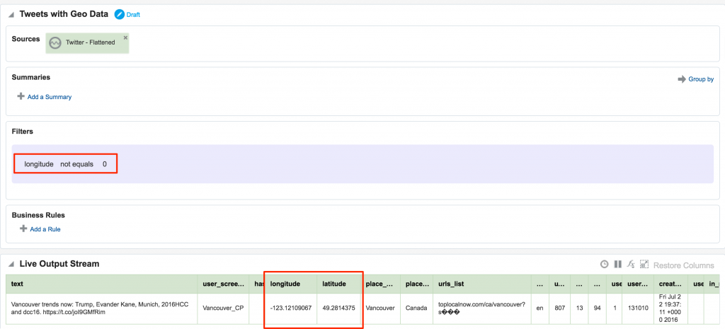
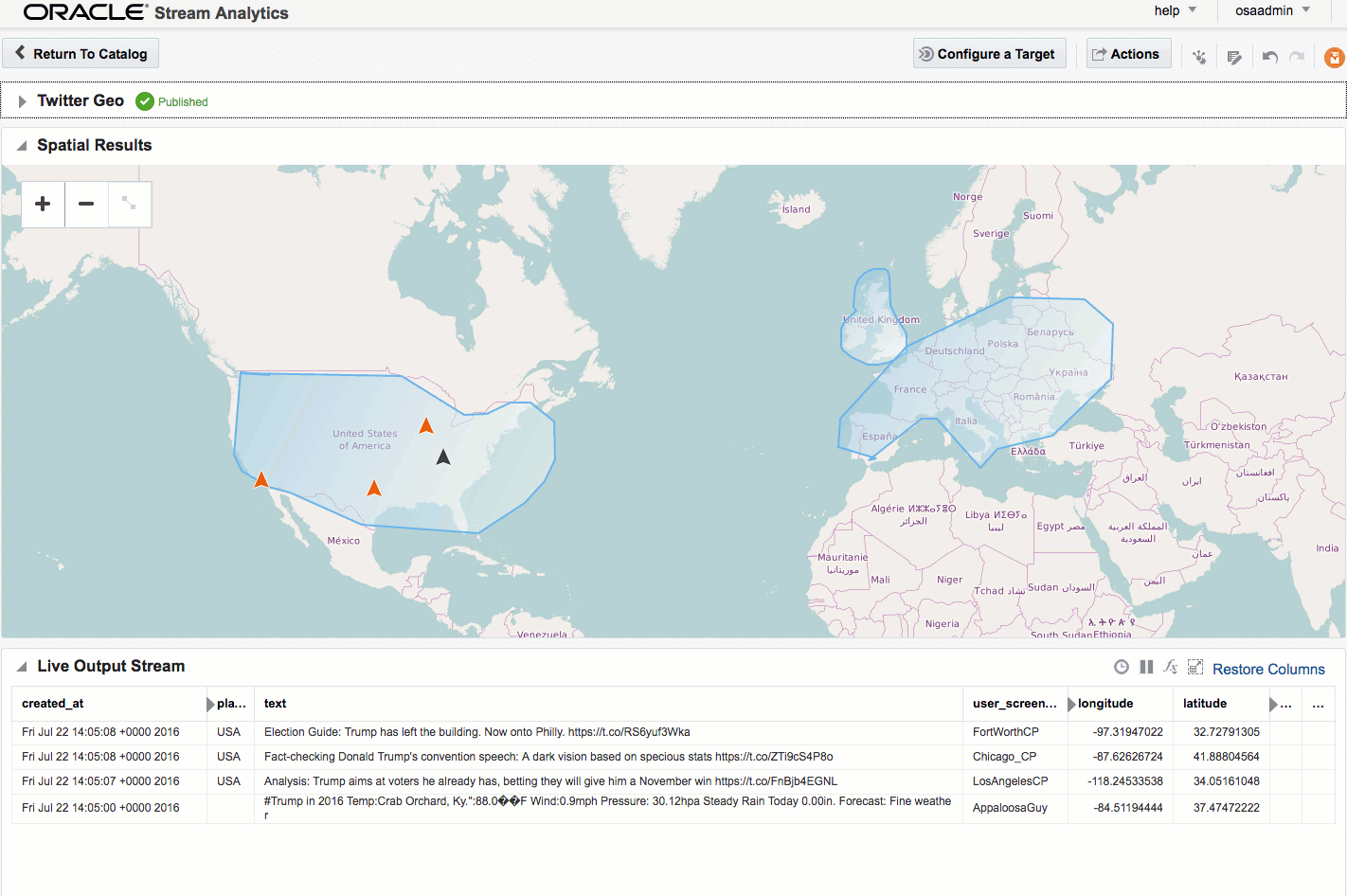
One of the Patterns that OSA provides is a Spatial one, which can be used to analyse source data that includes geo-location data. This could be to simply plot the occurrence of the data point (as we'll see shortly) on a map. It can also be used in a more sophisticated manner, to track a given entity's movements on a map. An example of this could be a fleet of trucks reporting their position back at regular intervals. Areas on a map can be defined and conditions triggered as the entity enters or leaves the area. For now though, we'll keep it simple. Using the flattened Twitter stream from Kafka that I produced from Logstash above, I'm going to plot Tweets in realtime on a map, along with a very simplistic tagging of the broad area in which they came from.
In my source Kafka topic I have two fields, latitude and longitude. I expose these as part of the 'flattening' of the JSON in this logstash script, since by default they're nested within the coordinates field and as an array too. When defining the Stream's Shape make sure you define the datatype correctly (Double) - OSA is not very forgiving of stupidity and I spent a frustrating time trying to work out why "-80.1422195" was coming through as zero - obviously defined as an Integer this was never going to work!
Not entirely necessary, but useful for debug purposes, I setup an exploration based on the flattened Twitter stream, with a filter to only include tweets that had geo-location data in them. This way I knew what tweets I should expect to be seeing in the next step. One of the things that I have found with OSA is that it has a tendency to fail silently; instead of throwing errors you'll just not get any data. By setting up the filter exploration I could at least debug things a bit more easily.
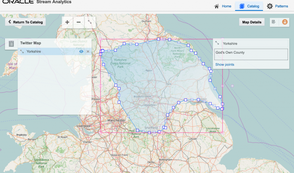
After this I created a new object, a Map. A Map object defines a set of named areas, which could be sourced from a database table, or drawn manually - which is what I did here by setting the Map Type to 'None (Create Manually)'. One thing to note about the maps is that they're sourced online (openstreetmap.org) so you'll need an internet connection to do this. Once the Map is open, click the Polygon Tool icon and click-drag a shape around the area that you want to "geo-fence". Each area is given a name, and this is what is used in the streaming data to label the event's geographical area.
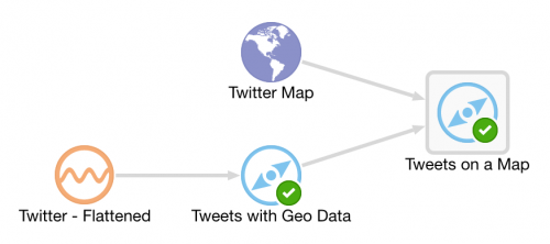
Having got our source data stream with geo-data in, and a Map on which to plot it and analyse the location of each event, we now use the Spatial General pattern to create an Exploration. The topology looks like this:
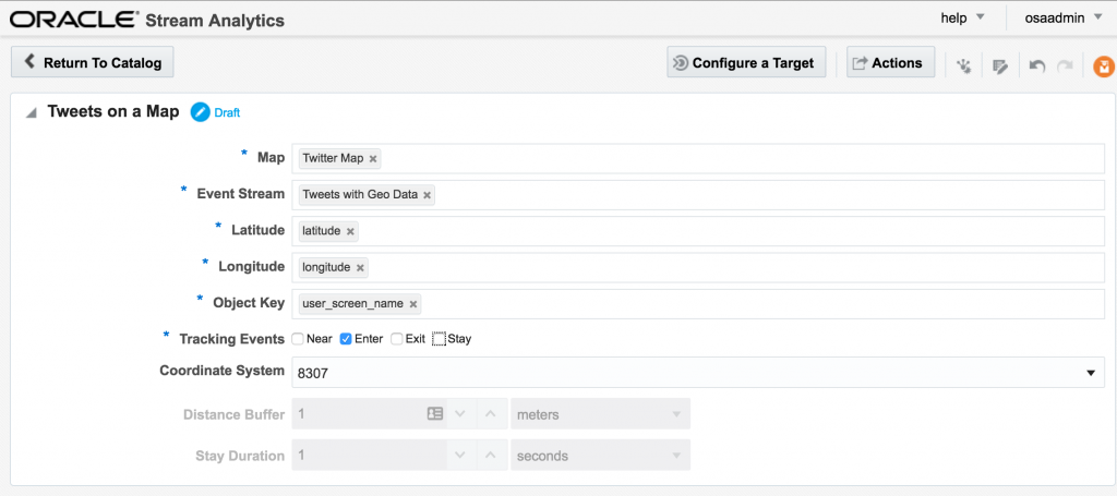
The fields in the Spatial General pattern are all pretty obvious. Object key is the field to use to track the same entity across multiple events, if you want to use the enter/exit/stay statuses. For tweets we just use 'Enter', but for people or vehicles, for example, you might get multiple status reports and want to track them on a map. For example, when a person is near a point of interest that you're tracking, or a vehicle has remained in a set area for too long.
If you let the Exploration now run, depending on the rate of event ingest, you'll sooner or later see points appearing on the map and event details underneath. The "status" column is populated (blank if the event is outside of the defined geo-fences), as is the "Place", based on the geo-fence names that you defined.
Summary
I can see OSA being used in two ways. The first as an ‘endpoint’ for streams with users taking actions based on the data, with some of the use cases listed here. The second is for prototyping transformations and analyses on streams prior to productionising them. The visual interface and immediacy of feedback on transformations applied means that users can quickly understand what further processing they may want to apply to the stream using actual streaming data to inform this.
This latter concept - that of prototyping - is similar to that which we see with another of Oracle’s products, Big Data Discovery. With BDD users can analyse data in the organisation’s data reservoir, as well as apply transformations to it (read more). Just as BDD doesn’t replace OBIEE or Visual Analyzer but enables users to understand how they do want to model the data in these tools, OSA wouldn’t replace “production grade” integration done by Oracle Data Integrator. What it would do is allow users to get a clearer idea of the transformations they would want performed in it.
OSA's user interface is easy to use and intuitive, and this is definitely a tool that you would put in front of technically minded business users. There are limitations to what can be achieved technically through the web GUI alone and something like Oracle Data Integrator (ODI) would still be a more appropriate fit for complex streaming work. At Oracle Open World last year it was announced (slides) that a beta would be starting for ODI using Spark Streaming for ETL and stream processing, so it'll be interesting to see this when it comes out.
Further Reading
- Providing Oracle Stream Analytics 12c environment using Docker, by Guido Schmutz
- Real-Time Data Streaming & Exploration with Oracle GoldenGate & Oracle Stream Analytics, by Issam Hijazi
- Demonstration of Oracle Stream Explorer for live device monitoring – collect, filter, aggregate, pattern match, enrich and publish by Lucas Jellema
- OTN OSA home page
- Documentation index
An Introduction to Oracle Stream Analytics
Oracle Stream Analytics (OSA) is a graphical tool that provides “Business Insight into Fast Data”. In layman terms, that translates into an intuitive web-based interface for exploring, analysing, and manipulating streaming data sources in realtime. These sources can include REST, JMS queues, as well as Kafka. The inclusion of Kafka opens OSA up to integration with many new-build data pipelines that use this as a backbone technology.

Previously known as Oracle Stream Explorer, it is part of the SOA component of Fusion Middleware (just as OBIEE and ODI are part of FMW too). In a recent blog it was positioned as “[…] part of Oracle Data Integration And Governance Platform.”. Its Big Data credentials include support for Kafka as source and target, as well as the option to execute across multiple nodes for scaling performance and capacity using Spark.
I’ve been exploring OSA from the comfort of my own Mac, courtesy of Docker and a Docker image for OSA created by Guido Schmutz. The benefits of Docker are many and covered elsewhere, but what I loved about it in this instance was that I didn’t have to download a VM that was 10s of GB. Nor did I have to spend time learning how to install OSA from scratch, which whilst interesting wasn’t a priority compared to just trying to tool out and seeing what it could do. [Update] it turns out that installation is a piece of cake, and the download is less than 1Gb … but in general the principle still stands – Docker is a great way to get up and running quickly with something
In this article we’ll take OSA for a spin, looking at some of the functionality and terminology, and then real examples of use with live Twitter data.
To start with, we sign in to Oracle Stream Analytics:

From here, click on the Catalog link, where a list of all the resources are listed. Some of these resource types include:
- Streams – definitions of sources of data such as Kafka, JMS, and a dummy data generator (event generator)
- Connections – Servers etc from which Streams are defined
- Explorations – front-end for seeing contents of Streams in realtime, as well as applying light transformations
- Targets – destination for transformed streams
Viewing Realtime Twitter Data with OSA
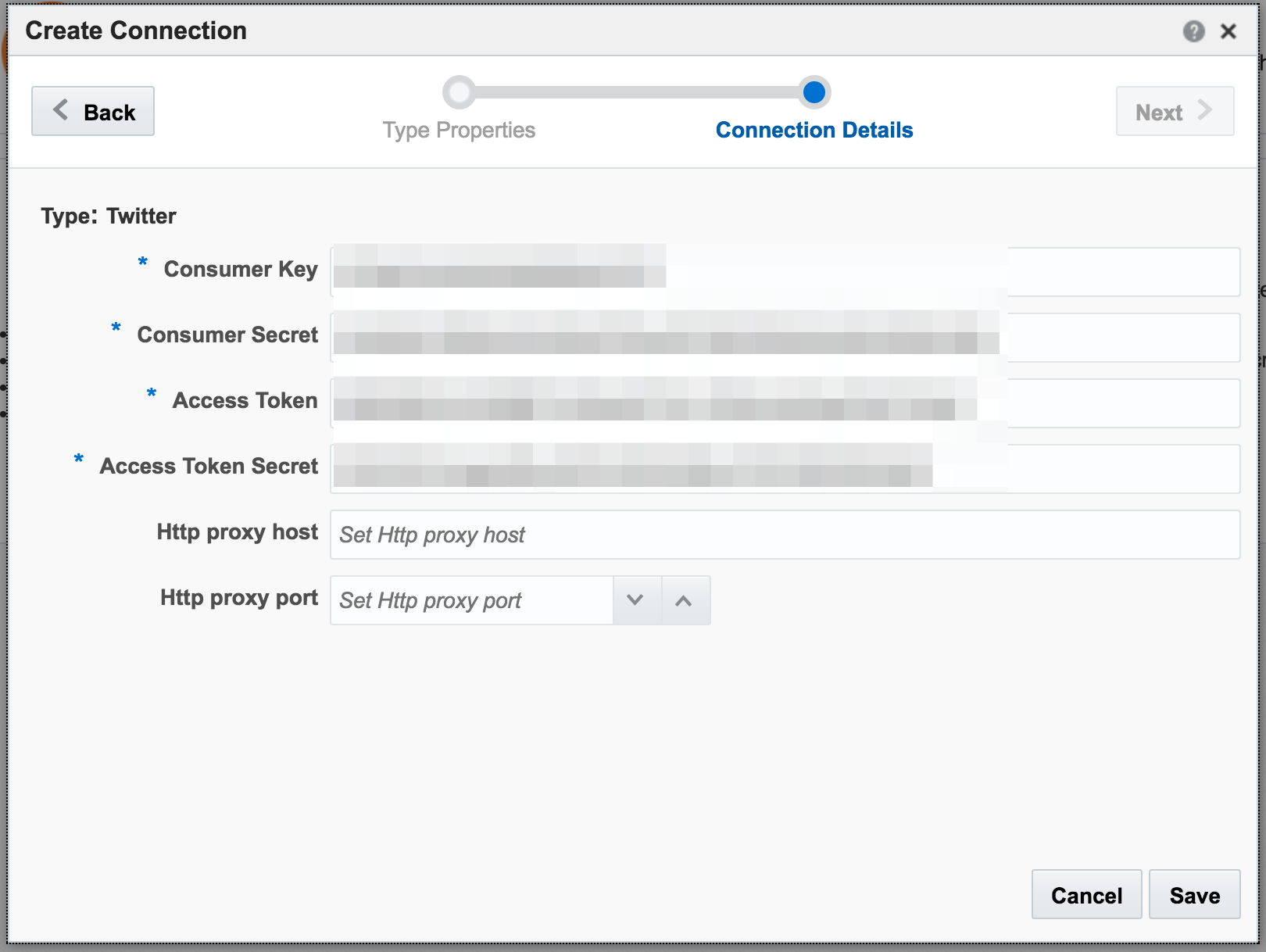
The first example I’ll show is the canonical big data/streaming example everywhere – Twitter. Twitter is even built into OSA as a Stream source. If you go to https://dev.twitter.com you can get yourself a set of credentials enabling you to query the live Twitter firehose for given hashtags or users.
With my twitter dev credentials, I create a new Connection in OSA:


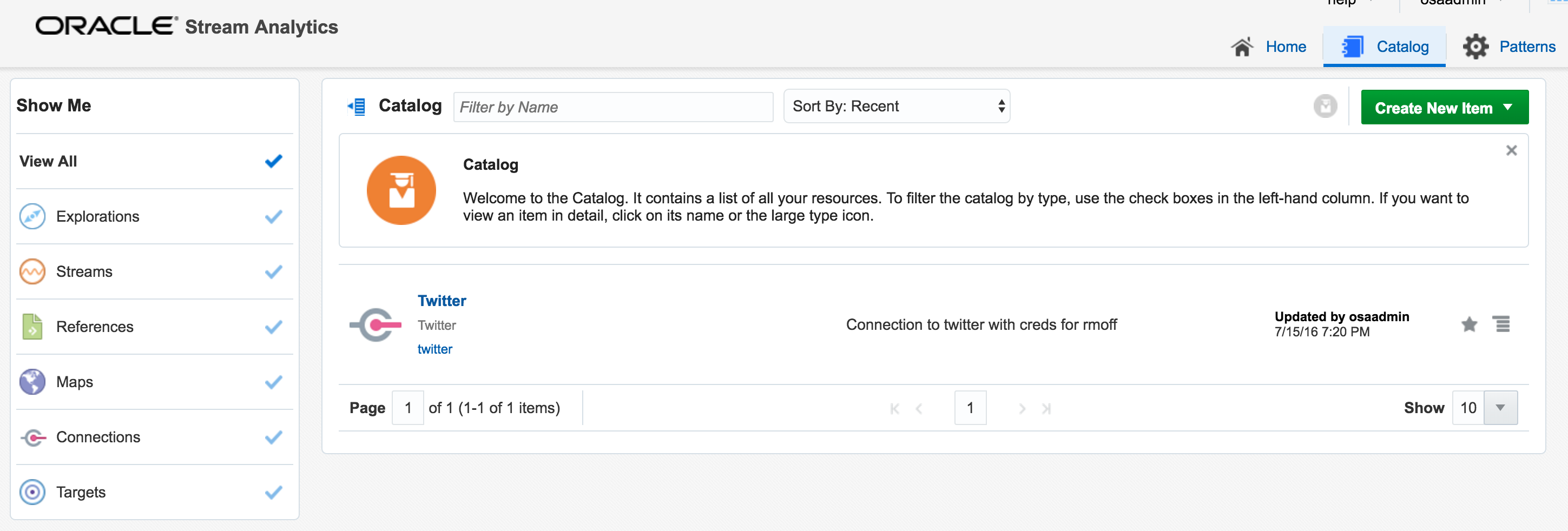
Now we have an entry in the Catalog, for the Twitter connection:

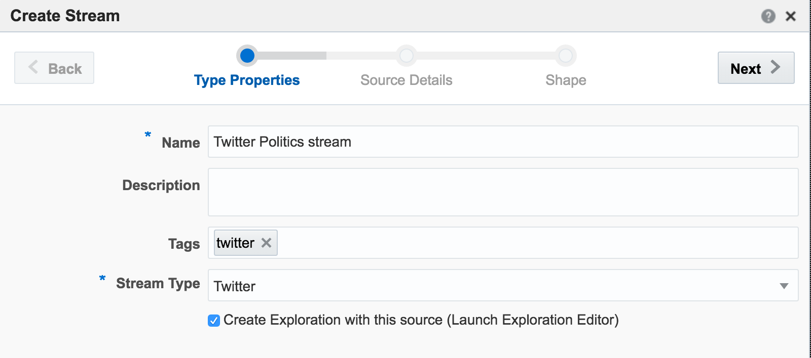
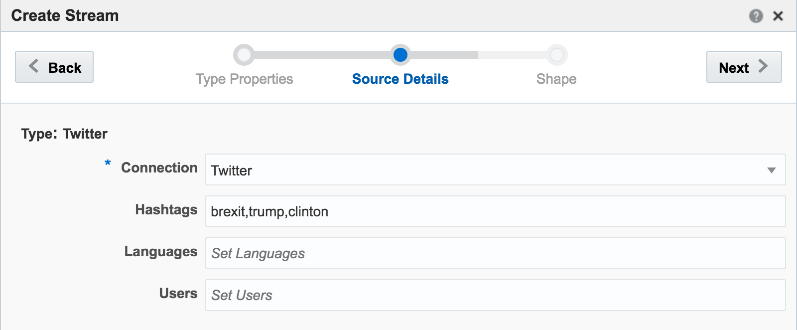
from which we can create a Stream, using the connection and a set of hashtags or users for whom we want to stream tweets:


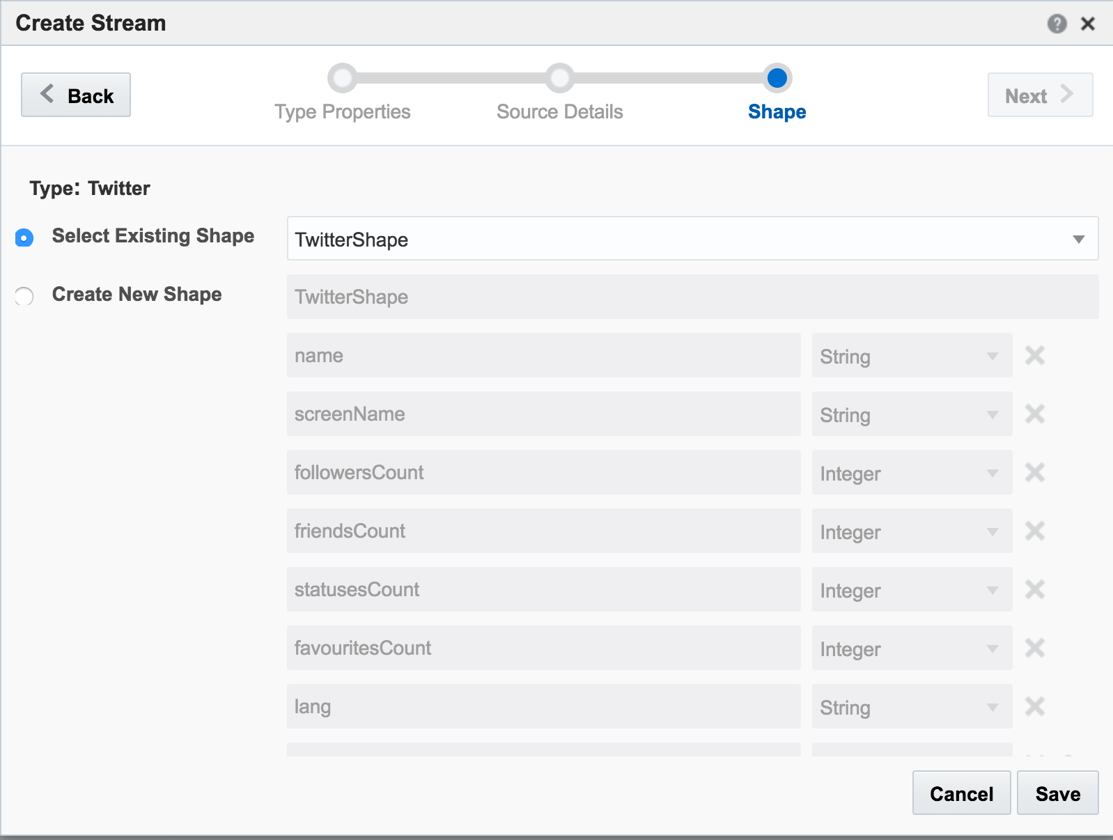
The Shape is basically the schema or data model that is applied for the stream. There is one built-in for Twitter, which we’ll use here:

When you click Save, if you get an error Unable to deploy OEP application then check the OSA log file for errors such as unable to reach Twitter, or invalid credentials.
Assuming the Stream is created successfully you are then prompted to create an Exploration from where you can see the Stream in realtime:

Explorations can have multiple stream sources, and be used to transform the contents, which we’ll see later. For now, after clicking Create, we get our Exploration window, which shows the contents of the stream in realtime:
At the bottom of the screen there’s the option to plot one or more charts showing the value of any numeric values in the stream, as can be seen in the animation above.
I’ll leave this example here for now, but finish by using the Publish option from the Actions menu, which makes it available as a source for subsequent analyses.
Adding Lookup Data to Streams
Let’s look now at some more of the options available for transforming and ‘wrangling’ streaming data with OSA. Here I’m going to show how two streams can be joined together (but not crossed) based on a common field, and the resulting stream used as the input for a subsequent process. The data is simulated, using a CSV file (read by OSA on a loop) and OSA’s Event Generator.
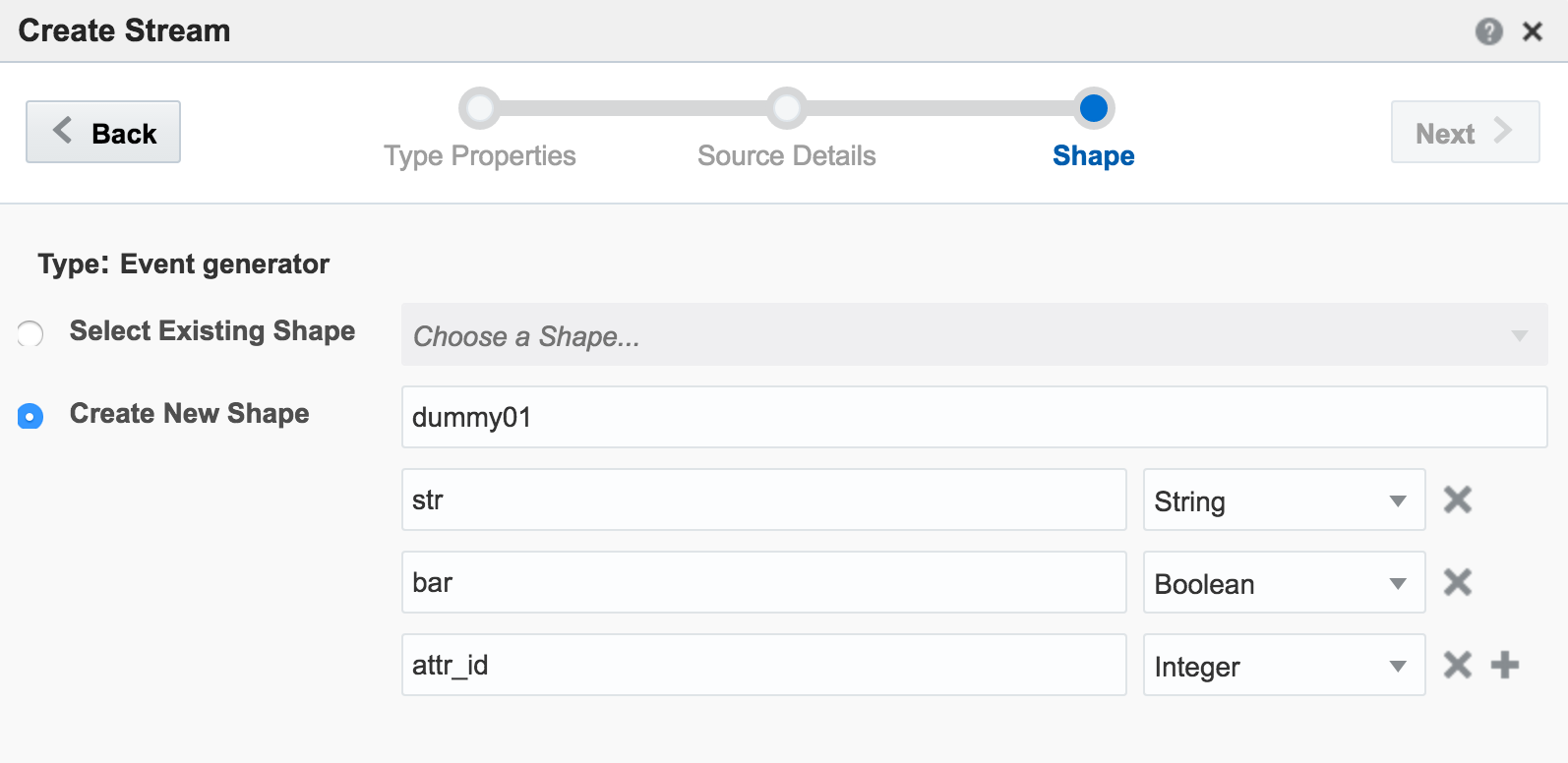
From the Catalog page I create a new Stream, using Event Generator as the Type:

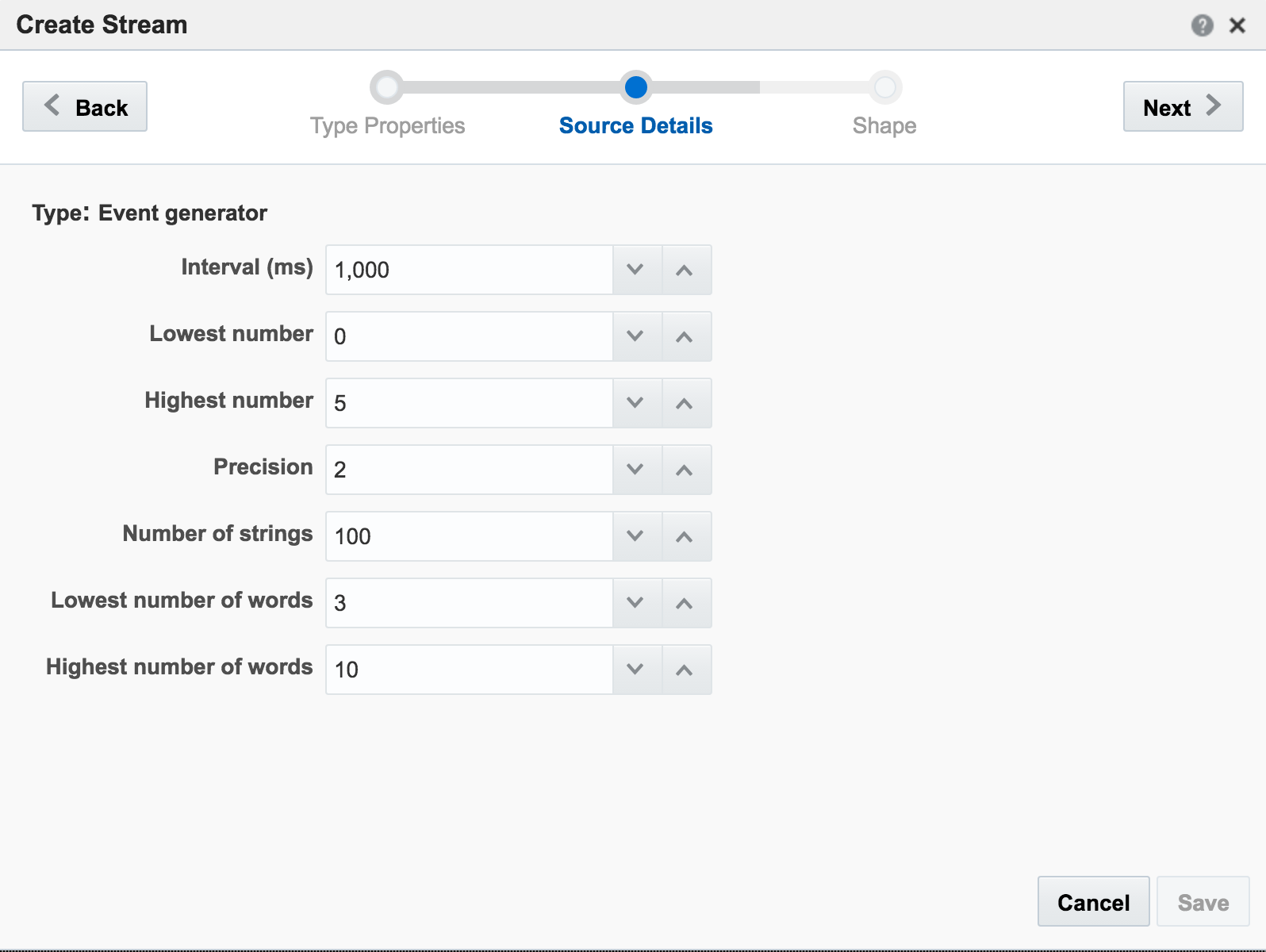
On the second page of the setup I define how frequently I want the dummy events to be generated, and the specification for the dummy data:

The last bit of setup for the stream is to define the Shape, which is the schema of data that I’d like generated:

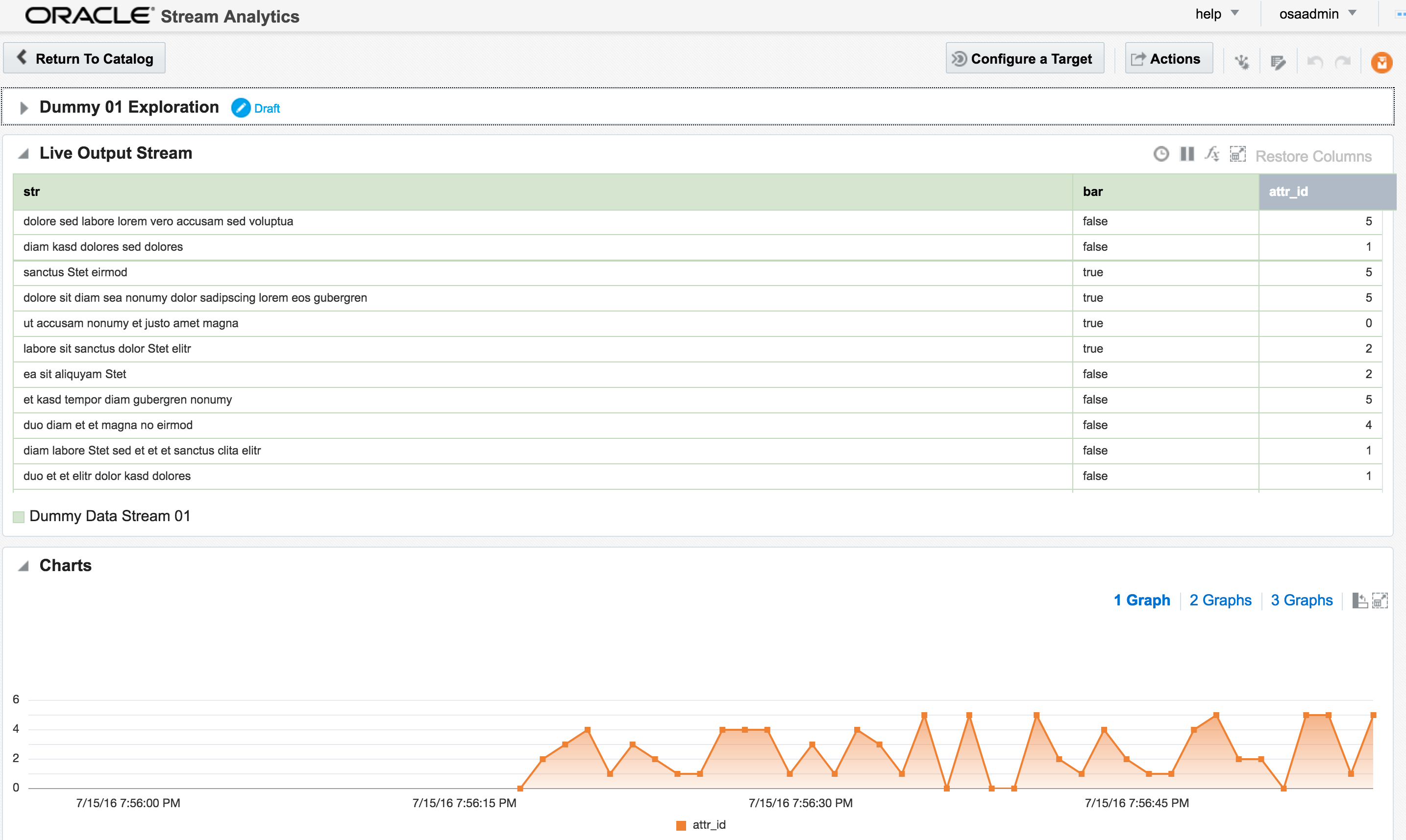
The Exploration for this stream shows the dummy data:

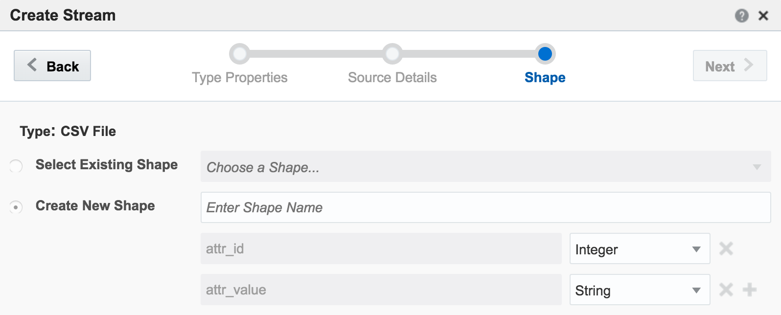
The second stream is going to be sourced from a very simple key/value CSV file:
attr_id,attr_value
1,never
2,gonna
3,give
4,you
5,up
The stream type is CSV, and I can configure how often OSA reads from it, as well as telling OSA to loop back to the beginning when it’s read to the end, thus simulating a proper stream. The ‘shape’ is picked up automatically from the file, based on the first row (headers) and then inferred data types:

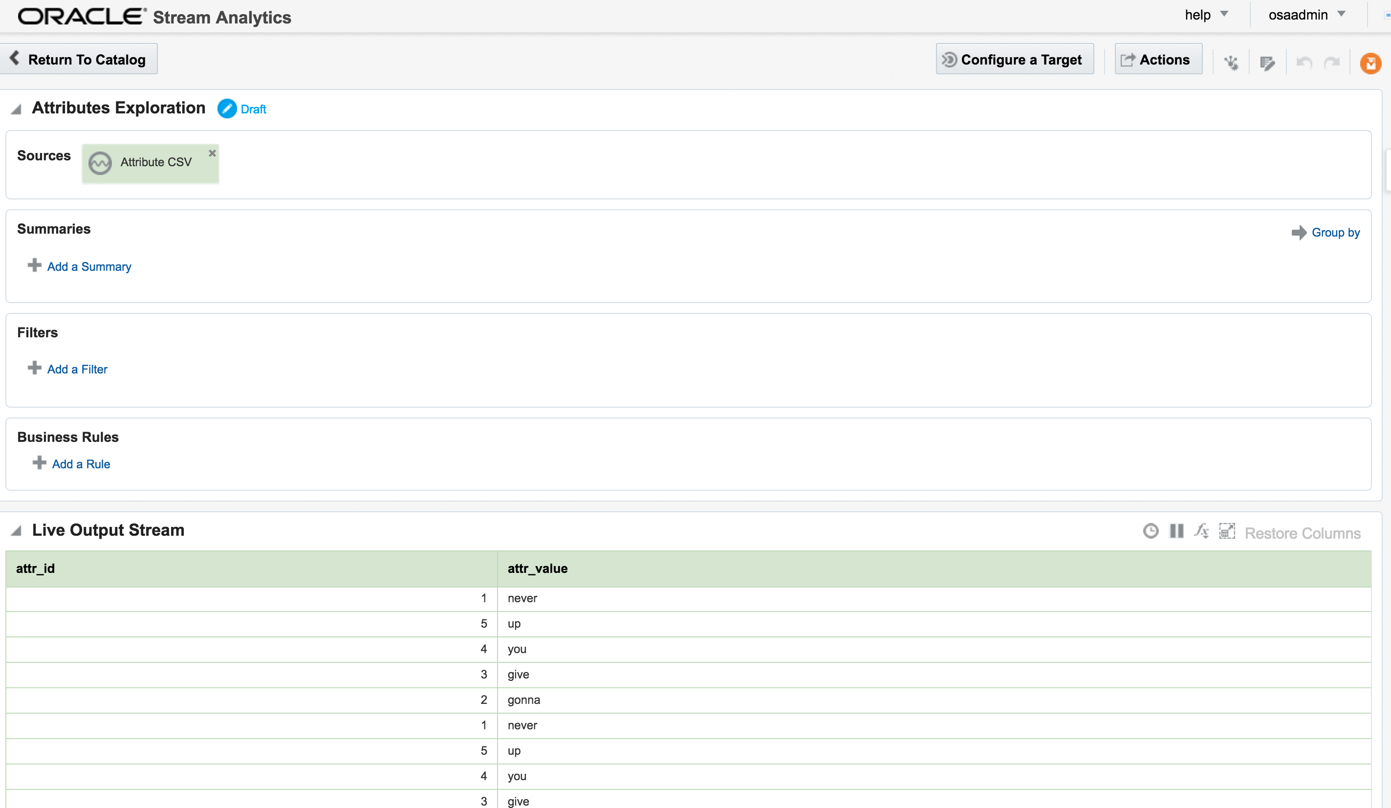
The Exploration for the stream shows the five values repeatedly streamed through (since I ticked the box to ‘loop’ the CSV file in the stream):

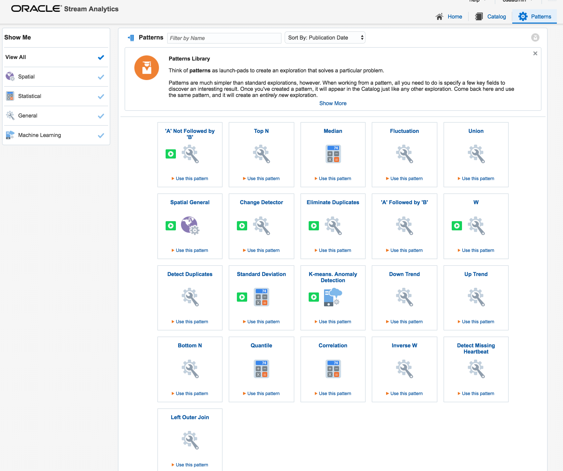
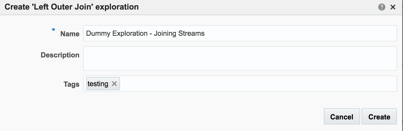
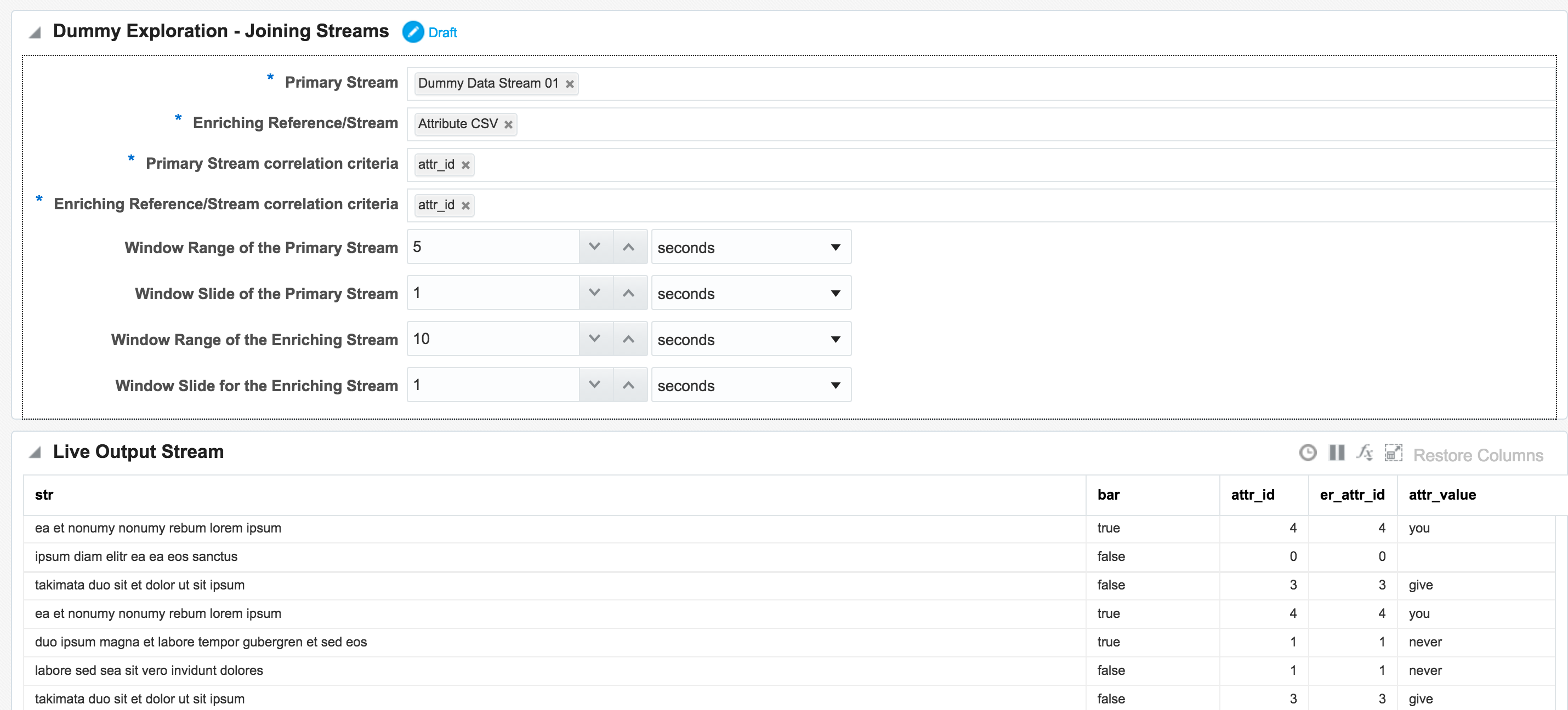
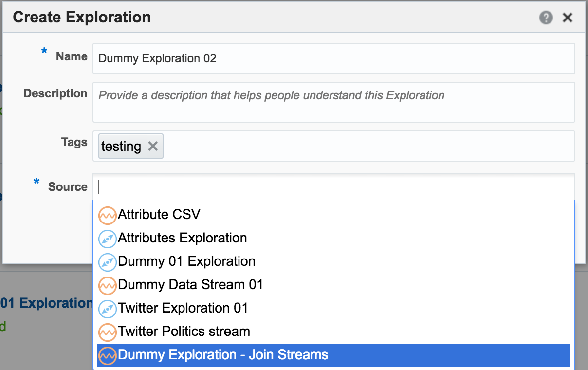
Back on the Catalog page I’m going to create a new Exploration, but this time based on a Pattern. Patterns are pre-built templates for stream manipulation and processing. Here we’ll use the pattern for a “left outer join” between streams.


The Pattern has a set of pre-defined fields that need to be supplied, including the stream names and the common field with which to join them. Note also that I’ve increased the Window Range. This is necessary so that a greater range of CSV stream events are used for the lookup. If the Range is left at the default of 1 second then only events from both streams occurring in the same second that match on attr_id would be matched. Unless both streams happen to be in sync on the same attr_id from the outset then this isn’t going to happen that often, and certainly wouldn’t in a real-life data stream.
So now we have the two joined streams:

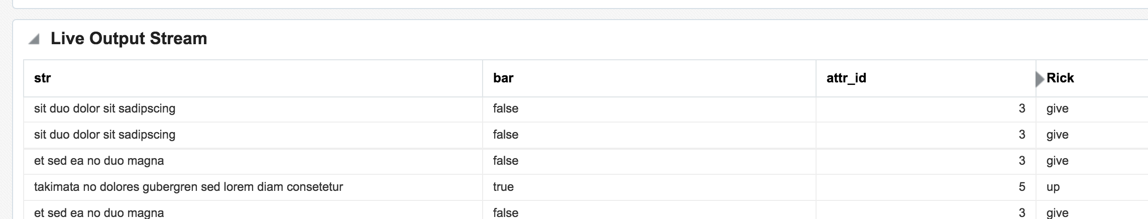
Within an Exploration it is possible to do light transformation work. By right-clicking on a column you can rename or remove it, which I’ve done here for the duplicated attr_id (duplicated since it appears in both streams), as well as renamed the attr_value:

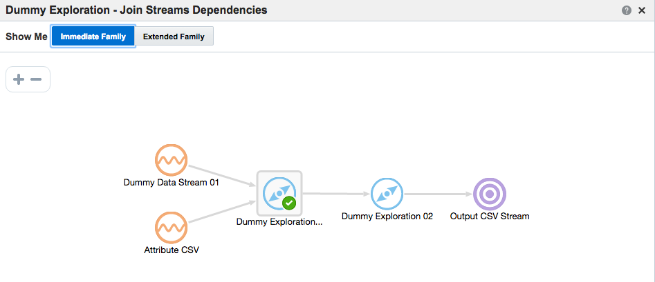
Daisy-Chaining, Targets, and Topology
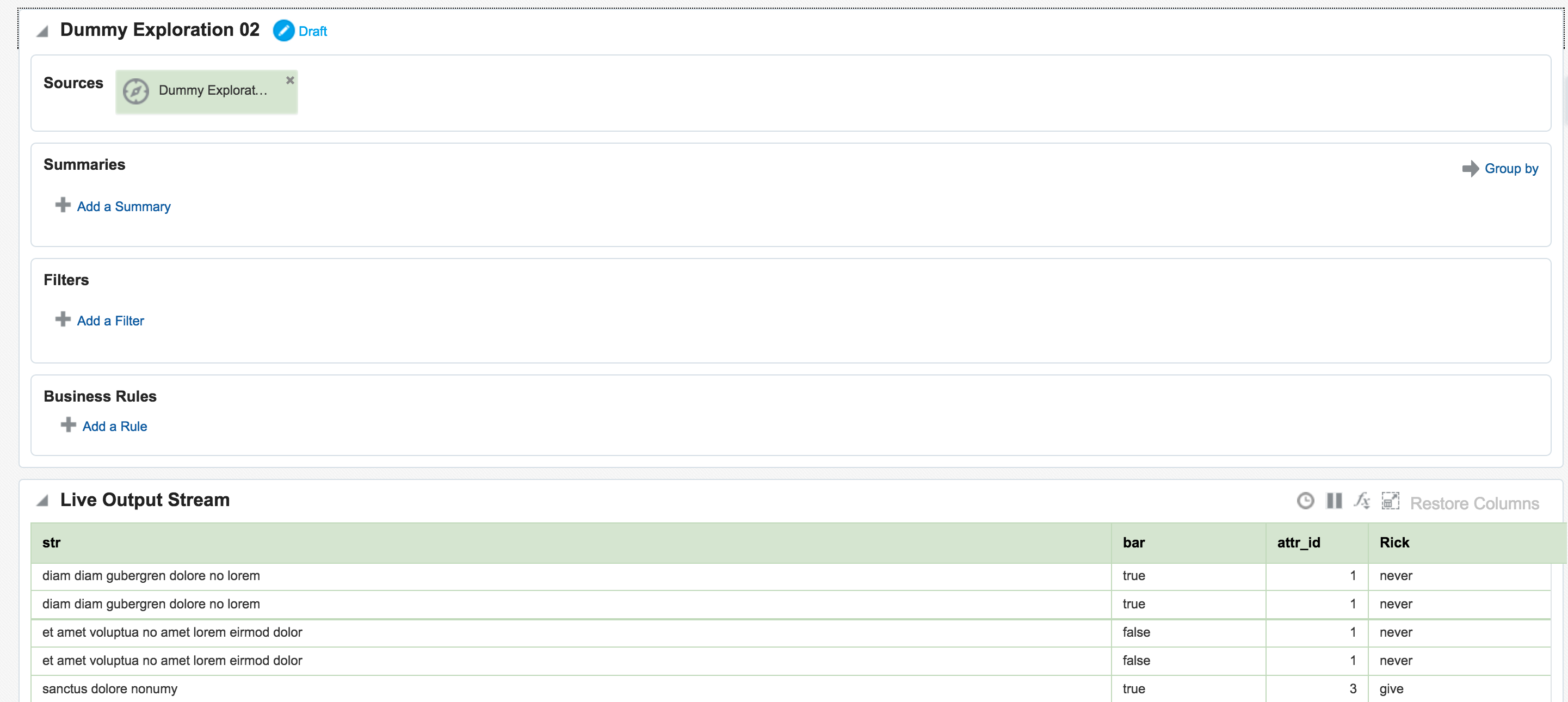
Once an Exploration is Published it can be used as the Source for subsequent Explorations, enabling you to map out a pipeline based on multiple source streams and transformations. Here we’re taking the exploration created just above that joined the two streams together, and using the output as the source for a new Exploration:

Since the Exploration is based on a previous one, the same stream data is available, but with the joins and transformations already applied

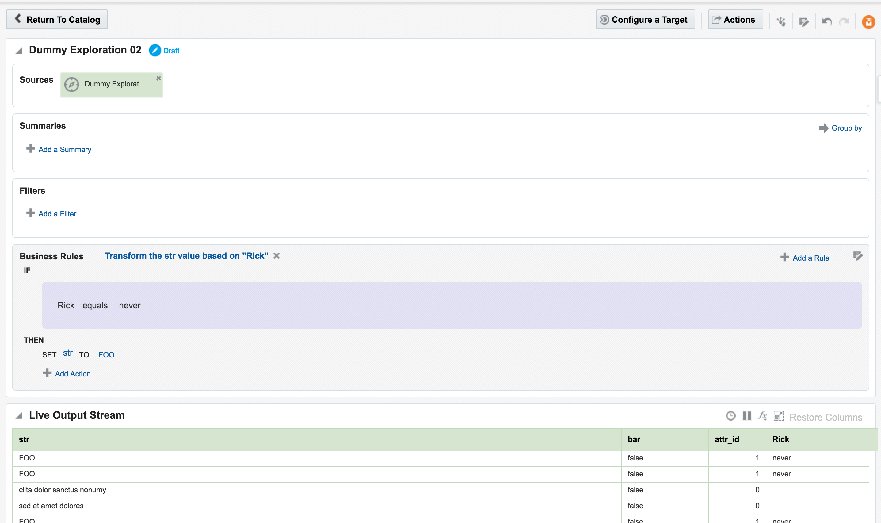
From here another transformation could be applied, such as replacing the value of one column conditionally based on that of another

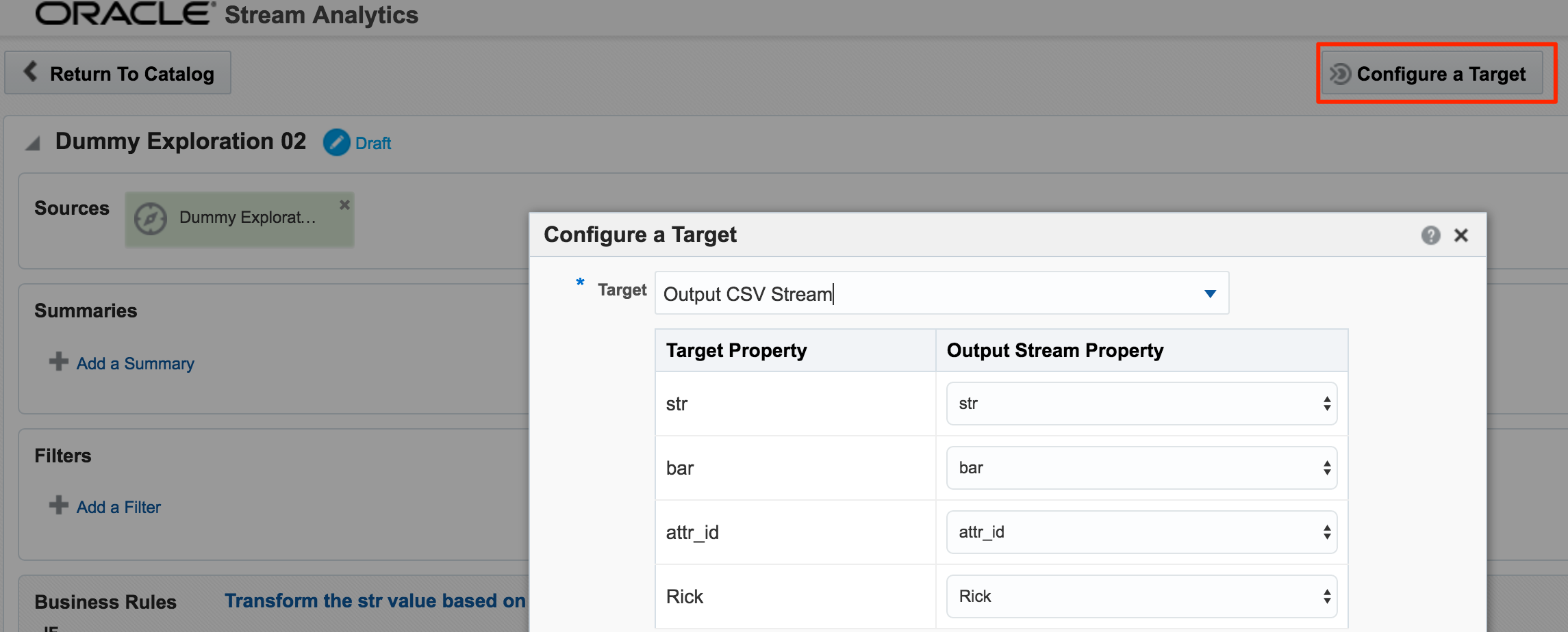
Whilst OSA enables rapid analysis and transformation of inbound streams, it also lets you stream the transformed results outside of OSA, to a Target as we saw in the Kafka example above. As well as Kafka other technologies are supported as targets, including a REST endpoint, or a simple CSV file.

With a target configured, as well as an Exploration based on the output of another, the Toplogy comes in handy for visualising the flow of data. You can access this from the Toplogy icon in an Exploration page, or from the dropdown menu on the Catalog page against a given object

In the next post I will look at how Oracle Stream Analytics can be used to analyse, enrich, and publish data to and from Kafka. Stay tuned!
The post An Introduction to Oracle Stream Analytics appeared first on Rittman Mead Consulting.
An Introduction to Oracle Stream Analytics

Oracle Stream Analytics (OSA) is a graphical tool that provides “Business Insight into Fast Data”. In layman terms, that translates into an intuitive web-based interface for exploring, analysing, and manipulating streaming data sources in realtime. These sources can include REST, JMS queues, as well as Kafka. The inclusion of Kafka opens OSA up to integration with many new-build data pipelines that use this as a backbone technology.

- Streams - definitions of sources of data such as Kafka, JMS, and a dummy data generator (event generator)
- Connections - Servers etc from which Streams are defined
- Explorations - front-end for seeing contents of Streams in realtime, as well as applying light transformations
- Targets - destination for transformed streams
Viewing Realtime Twitter Data with OSA
The first example I’ll show is the canonical big data/streaming example everywhere – Twitter. Twitter is even built into OSA as a Stream source. If you go to https://dev.twitter.com you can get yourself a set of credentials enabling you to query the live Twitter firehose for given hashtags or users. With my twitter dev credentials, I create a new Connection in OSA: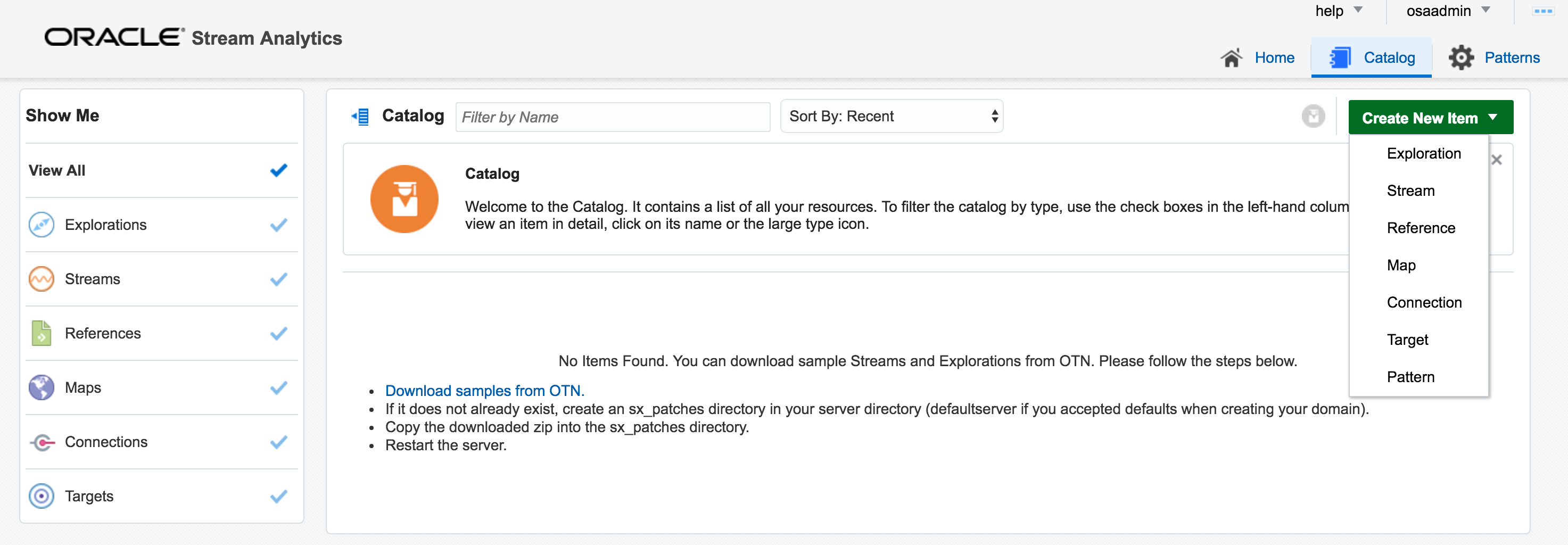
Unable to deploy OEP application then check the OSA log file for errors such as unable to reach Twitter, or invalid credentials.
Assuming the Stream is created successfully you are then prompted to create an Exploration from where you can see the Stream in realtime:
Adding Lookup Data to Streams
Let's look now at some more of the options available for transforming and 'wrangling' streaming data with OSA. Here I’m going to show how two streams can be joined together (but not crossed) based on a common field, and the resulting stream used as the input for a subsequent process. The data is simulated, using a CSV file (read by OSA on a loop) and OSA's Event Generator. From the Catalog page I create a new Stream, using Event Generator as the Type: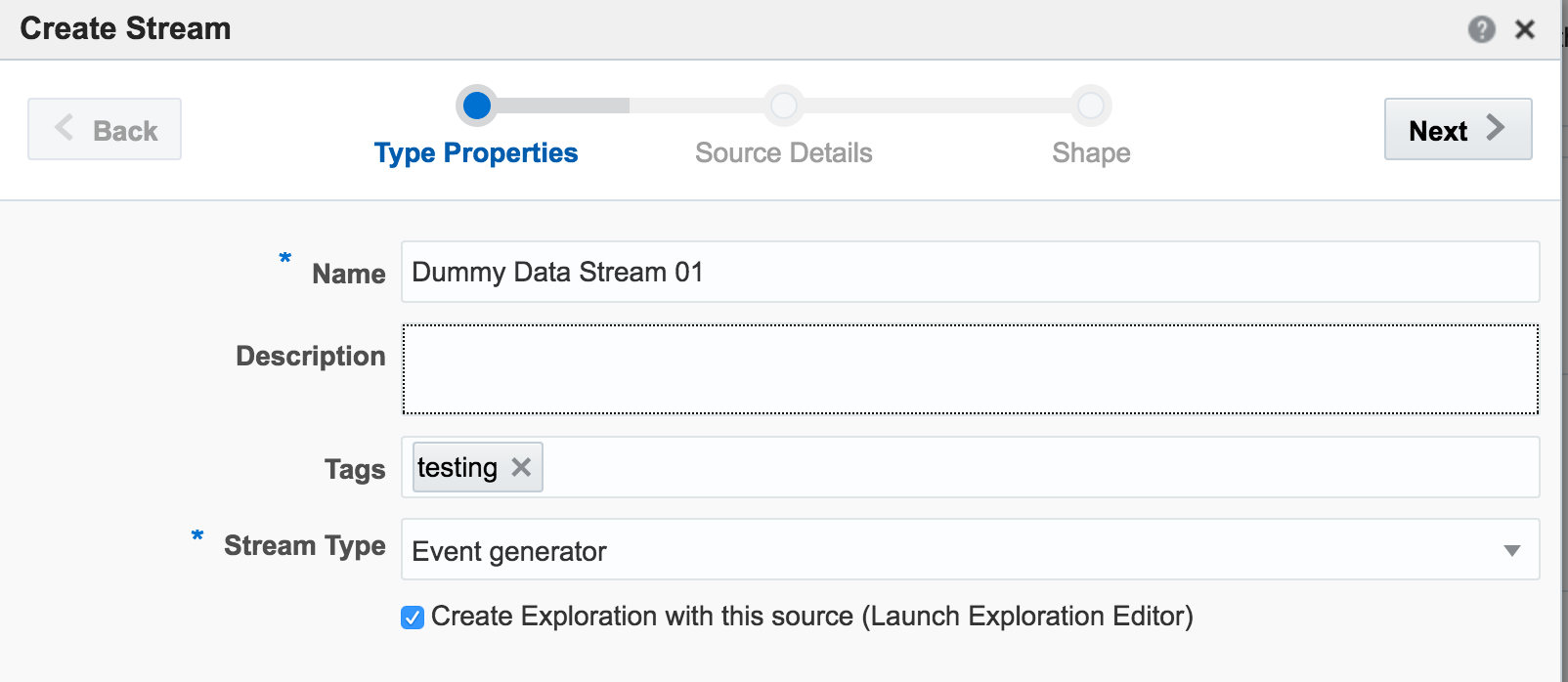
attr_id,attr_value
1,never
2,gonna
3,give
4,you
5,up
The stream type is CSV, and I can configure how often OSA reads from it, as well as telling OSA to loop back to the beginning when it's read to the end, thus simulating a proper stream. The ‘shape’ is picked up automatically from the file, based on the first row (headers) and then inferred data types:
attr_id would be matched. Unless both streams happen to be in sync on the same attr_id from the outset then this isn’t going to happen that often, and certainly wouldn’t in a real-life data stream.
So now we have the two joined streams:
attr_id (duplicated since it appears in both streams), as well as renamed the attr_value:
Daisy-Chaining, Targets, and Topology
Once an Exploration is Published it can be used as the Source for subsequent Explorations, enabling you to map out a pipeline based on multiple source streams and transformations. Here we're taking the exploration created just above that joined the two streams together, and using the output as the source for a new Exploration:
In the next post I will look at how Oracle Stream Analytics can be used to analyse, enrich, and publish data to and from Kafka. Stay tuned!
Using R with Jupyter Notebooks and Big Data Discovery
Oracle’s Big Data Discovery encompasses a good amount of exploration, transformation, and visualisation capabilities for datasets residing in your organisation’s data reservoir. Even with this though, there may come a time when your data scientists want to unleash their R magic on those same datasets. Perhaps the data domain expert has used BDD to enrich and cleanse the data, and now it’s ready for some statistical analysis? Maybe you’d like to use R’s excellent forecast package to predict the next six months of a KPI from the BDD dataset? And not only predict it, but write it back into the dataset for subsequent use in BDD? This is possible using BDD Shell and rpy2. It enables advanced analysis and manipulation of datasets already in BDD. These modified datasets can then be pushed back into Hive and then BDD.
BDD Shell provides a native Python environment, and you may opt to use the pandas library to work with BDD datasets as detailed here. In other cases you may simply prefer working with R, or have a particular library in mind that only R offers natively. In this article we’ll see how to do that. The “secret sauce” is rpy2 which enables the native use of R code within a python-kernel Jupyter Notebook.
As with previous articles I’m using a Jupyter Notebook as my environment. I’ll walk through the code here, and finish with a copy of the notebook so you can see the full process.
First we’ll see how you can use R in Jupyter Notebooks running a python kernel, and then expand out to integrate with BDD too. You can view and download the first notebook here.
Import the RPY2 environment so that we can call R from Jupyter
import readline is necessary to workaround the error: /u01/anaconda2/lib/libreadline.so.6: undefined symbol: PC
import readline
%load_ext rpy2.ipython
Example usage
Single inline command, prefixed with %R
%R X=c(1,4,5,7); sd(X); mean(X)
array([ 4.25])
R code block, marked by %%R
%%R
Y = c(2,4,3,9)
summary(lm(Y~X))
Call:
lm(formula = Y ~ X)

Residuals:
    1     2     3     4
 0.88 -0.24 -2.28  1.64

Coefficients:
            Estimate Std. Error t value Pr(>|t|)
(Intercept)   0.0800     2.3000   0.035    0.975
X             1.0400     0.4822   2.157    0.164

Residual standard error: 2.088 on 2 degrees of freedom
Multiple R-squared:  0.6993,    Adjusted R-squared:  0.549
F-statistic: 4.651 on 1 and 2 DF,  p-value: 0.1638
Graphics plot, output to the notebook
%R plot(X, Y)

Pass Python variable to R using -i
import numpy as np
Z = np.array([1,4,5,10])
%R -i Z mean(Z)
array([ 5.])
For more information see the documentation
Working with BDD Datasets from R in Jupyter Notebooks
Now that we’ve seen calling R in Jupyter Notebooks, let’s see how to use it with BDD in order to access datasets. The first step is to instantiate the BDD Shell so that you can access the datasets in BDD, and then to set up the R environment using rpy2
execfile('ipython/00-bdd-shell-init.py')
%load_ext rpy2.ipython
I also found that I had to make readline available otherwise I got an error (/u01/anaconda2/lib/libreadline.so.6: undefined symbol: PC)
import readline
After this, we can import a BDD dataset, convert it to a Spark dataframe and then a pandas dataframe, ready for passing to R
ds = dss.dataset('edp_cli_edp_8d6fd230-8e99-449c-9480-0c2bddc4f6dc')
spark_df = ds.to_spark()
import pandas as pd
pandas_df = spark_df.toPandas()
Note that there is a lot of passing of the same dataframe into different memory structures here – from BDD dataset context to Spark to Pandas, and that’s before we’ve even hit R. It’s fine for ad-hoc wrangling but might start to be painful with very large datasets.
Now we use the rpy2 integration with Jupyter Notebooks and invoke R parsing of the cell’s contents, using the %%R syntax. Optionally, we can pass across variables with the -i parameter, which we’re doing here. Then we assign the dataframe to an R-notation variable (optional, but stylistically nice to do), and then use R’s summary function to show a summary of each attribute:
%%R -i pandas_df
R.df <- pandas_df
summary(R.df)
vendorid     tpep_pickup_datetime tpep_dropoff_datetime passenger_count
 Min.   :1.000   Min.   :1.420e+12    Min.   :1.420e+12     Min.   :0.000
 1st Qu.:1.000   1st Qu.:1.427e+12    1st Qu.:1.427e+12     1st Qu.:1.000
 Median :2.000   Median :1.435e+12    Median :1.435e+12     Median :1.000
 Mean   :1.525   Mean   :1.435e+12    Mean   :1.435e+12     Mean   :1.679
 3rd Qu.:2.000   3rd Qu.:1.443e+12    3rd Qu.:1.443e+12     3rd Qu.:2.000
 Max.   :2.000   Max.   :1.452e+12    Max.   :1.452e+12     Max.   :9.000
 NA's   :12      NA's   :12           NA's   :12            NA's   :12
 trip_distance      pickup_longitude  pickup_latitude    ratecodeid
 Min.   :    0.00   Min.   :-121.93   Min.   :-58.43   Min.   : 1.000
 1st Qu.:    1.00   1st Qu.: -73.99   1st Qu.: 40.74   1st Qu.: 1.000
 Median :    1.71   Median : -73.98   Median : 40.75   Median : 1.000
 Mean   :    3.04   Mean   : -72.80   Mean   : 40.10   Mean   : 1.041
 3rd Qu.:    3.20   3rd Qu.: -73.97   3rd Qu.: 40.77   3rd Qu.: 1.000
 Max.   :67468.40   Max.   : 133.82   Max.   : 62.77   Max.   :99.000
 NA's   :12         NA's   :12        NA's   :12       NA's   :12
 store_and_fwd_flag dropoff_longitude dropoff_latitude  payment_type
 N   :992336        Min.   :-121.93   Min.   : 0.00    Min.   :1.00
 None:    12        1st Qu.: -73.99   1st Qu.:40.73    1st Qu.:1.00
 Y   :  8218        Median : -73.98   Median :40.75    Median :1.00
                    Mean   : -72.85   Mean   :40.13    Mean   :1.38
                    3rd Qu.: -73.96   3rd Qu.:40.77    3rd Qu.:2.00
                    Max.   :   0.00   Max.   :44.56    Max.   :5.00
                    NA's   :12        NA's   :12       NA's   :12
  fare_amount          extra            mta_tax          tip_amount
 Min.   :-170.00   Min.   :-1.0000   Min.   :-1.7000   Min.   :  0.000
 1st Qu.:   6.50   1st Qu.: 0.0000   1st Qu.: 0.5000   1st Qu.:  0.000
 Median :   9.50   Median : 0.0000   Median : 0.5000   Median :  1.160
 Mean   :  12.89   Mean   : 0.3141   Mean   : 0.4977   Mean   :  1.699
 3rd Qu.:  14.50   3rd Qu.: 0.5000   3rd Qu.: 0.5000   3rd Qu.:  2.300
 Max.   : 750.00   Max.   :49.6000   Max.   :52.7500   Max.   :360.000
 NA's   :12        NA's   :12        NA's   :12        NA's   :12
  tolls_amount      improvement_surcharge  total_amount       PRIMARY_KEY
 Min.   : -5.5400   Min.   :-0.3000       Min.   :-170.80   0-0-0   :      1
 1st Qu.:  0.0000   1st Qu.: 0.3000       1st Qu.:   8.75   0-0-1   :      1
 Median :  0.0000   Median : 0.3000       Median :  11.80   0-0-10  :      1
 Mean   :  0.3072   Mean   : 0.2983       Mean   :  16.01   0-0-100 :      1
 3rd Qu.:  0.0000   3rd Qu.: 0.3000       3rd Qu.:  17.80   0-0-1000:      1
 Max.   :503.0500   Max.   : 0.3000       Max.   : 760.05   0-0-1001:      1
 NA's   :12         NA's   :12            NA's   :12        (Other) :1000560
We can use native R code and R libraries including the excellent dplyr to lightly wrangle and then chart the data:
%%R

library(dplyr)
library(ggplot2)

R.df %>%
    filter(fare_amount > 0) %>%
    ggplot(aes(y=fare_amount, x=tip_amount,color=passenger_count)) +
    geom_point(alpha=0.5 )

Finally, using the -o flag on the %%R invocation, we can pass back variables from the R context back to pandas :
%%R -o R_output
R_output <-
    R.df %>%
    mutate(foo = 'bar')
and from there back to Spark and write the results to Hive:
spark_df2 = sqlContext.createDataFrame(R_output)
spark_df2.write.mode('Overwrite').saveAsTable('default.updated_dataset')
and finally ingest the new Hive table to BDD:
from subprocess import call
call(["/u01/bdd/v1.2.0/BDD-1.2.0.31.813/dataprocessing/edp_cli/data_processing_CLI","--table default.updated_dataset"])
You can download the notebook here.
The post Using R with Jupyter Notebooks and Big Data Discovery appeared first on Rittman Mead Consulting.
Using R with Jupyter Notebooks and Big Data Discovery
Oracle’s Big Data Discovery encompasses a good amount of exploration, transformation, and visualisation capabilities for datasets residing in your organisation’s data reservoir. Even with this though, there may come a time when your data scientists want to unleash their R magic on those same datasets. Perhaps the data domain expert has used BDD to enrich and cleanse the data, and now it’s ready for some statistical analysis? Maybe you’d like to use R’s excellent forecast package to predict the next six months of a KPI from the BDD dataset? And not only predict it, but write it back into the dataset for subsequent use in BDD? This is possible using BDD Shell and rpy2. It enables advanced analysis and manipulation of datasets already in BDD. These modified datasets can then be pushed back into Hive and then BDD.
BDD Shell provides a native Python environment, and you may opt to use the pandas library to work with BDD datasets as detailed here. In other cases you may simply prefer working with R, or have a particular library in mind that only R offers natively. In this article we’ll see how to do that. The “secret sauce” is rpy2 which enables the native use of R code within a python-kernel Jupyter Notebook.
As with previous articles I’m using a Jupyter Notebook as my environment. I’ll walk through the code here, and finish with a copy of the notebook so you can see the full process.
First we’ll see how you can use R in Jupyter Notebooks running a python kernel, and then expand out to integrate with BDD too. You can view and download the first notebook here.
Import the RPY2 environment so that we can call R from Jupyter
import readline is necessary to workaround the error: /u01/anaconda2/lib/libreadline.so.6: undefined symbol: PC
import readline
%load_ext rpy2.ipython
Example usage
Single inline command, prefixed with %R
%R X=c(1,4,5,7); sd(X); mean(X)
array([ 4.25])
R code block, marked by %%R
%%R
Y = c(2,4,3,9)
summary(lm(Y~X))
Call:
lm(formula = Y ~ X)

Residuals:
    1     2     3     4
 0.88 -0.24 -2.28  1.64

Coefficients:
            Estimate Std. Error t value Pr(>|t|)
(Intercept)   0.0800     2.3000   0.035    0.975
X             1.0400     0.4822   2.157    0.164

Residual standard error: 2.088 on 2 degrees of freedom
Multiple R-squared:  0.6993,    Adjusted R-squared:  0.549
F-statistic: 4.651 on 1 and 2 DF,  p-value: 0.1638
Graphics plot, output to the notebook
%R plot(X, Y)
Pass Python variable to R using -i
import numpy as np
Z = np.array([1,4,5,10])
%R -i Z mean(Z)
array([ 5.])
For more information see the documentation
Working with BDD Datasets from R in Jupyter Notebooks
Now that we’ve seen calling R in Jupyter Notebooks, let’s see how to use it with BDD in order to access datasets. The first step is to instantiate the BDD Shell so that you can access the datasets in BDD, and then to set up the R environment using rpy2
execfile('ipython/00-bdd-shell-init.py')
%load_ext rpy2.ipython
I also found that I had to make readline available otherwise I got an error (/u01/anaconda2/lib/libreadline.so.6: undefined symbol: PC)
import readline
After this, we can import a BDD dataset, convert it to a Spark dataframe and then a pandas dataframe, ready for passing to R
ds = dss.dataset('edp_cli_edp_8d6fd230-8e99-449c-9480-0c2bddc4f6dc')
spark_df = ds.to_spark()
import pandas as pd
pandas_df = spark_df.toPandas()
Note that there is a lot of passing of the same dataframe into different memory structures here – from BDD dataset context to Spark to Pandas, and that’s before we’ve even hit R. It’s fine for ad-hoc wrangling but might start to be painful with very large datasets.
Now we use the rpy2 integration with Jupyter Notebooks and invoke R parsing of the cell’s contents, using the %%R syntax. Optionally, we can pass across variables with the -i parameter, which we’re doing here. Then we assign the dataframe to an R-notation variable (optional, but stylistically nice to do), and then use R’s summary function to show a summary of each attribute:
%%R -i pandas_df
R.df <- pandas_df
summary(R.df)
vendorid     tpep_pickup_datetime tpep_dropoff_datetime passenger_count
 Min.   :1.000   Min.   :1.420e+12    Min.   :1.420e+12     Min.   :0.000
 1st Qu.:1.000   1st Qu.:1.427e+12    1st Qu.:1.427e+12     1st Qu.:1.000
 Median :2.000   Median :1.435e+12    Median :1.435e+12     Median :1.000
 Mean   :1.525   Mean   :1.435e+12    Mean   :1.435e+12     Mean   :1.679
 3rd Qu.:2.000   3rd Qu.:1.443e+12    3rd Qu.:1.443e+12     3rd Qu.:2.000
 Max.   :2.000   Max.   :1.452e+12    Max.   :1.452e+12     Max.   :9.000
 NA's   :12      NA's   :12           NA's   :12            NA's   :12
 trip_distance      pickup_longitude  pickup_latitude    ratecodeid
 Min.   :    0.00   Min.   :-121.93   Min.   :-58.43   Min.   : 1.000
 1st Qu.:    1.00   1st Qu.: -73.99   1st Qu.: 40.74   1st Qu.: 1.000
 Median :    1.71   Median : -73.98   Median : 40.75   Median : 1.000
 Mean   :    3.04   Mean   : -72.80   Mean   : 40.10   Mean   : 1.041
 3rd Qu.:    3.20   3rd Qu.: -73.97   3rd Qu.: 40.77   3rd Qu.: 1.000
 Max.   :67468.40   Max.   : 133.82   Max.   : 62.77   Max.   :99.000
 NA's   :12         NA's   :12        NA's   :12       NA's   :12
 store_and_fwd_flag dropoff_longitude dropoff_latitude  payment_type
 N   :992336        Min.   :-121.93   Min.   : 0.00    Min.   :1.00
 None:    12        1st Qu.: -73.99   1st Qu.:40.73    1st Qu.:1.00
 Y   :  8218        Median : -73.98   Median :40.75    Median :1.00
                    Mean   : -72.85   Mean   :40.13    Mean   :1.38
                    3rd Qu.: -73.96   3rd Qu.:40.77    3rd Qu.:2.00
                    Max.   :   0.00   Max.   :44.56    Max.   :5.00
                    NA's   :12        NA's   :12       NA's   :12
  fare_amount          extra            mta_tax          tip_amount
 Min.   :-170.00   Min.   :-1.0000   Min.   :-1.7000   Min.   :  0.000
 1st Qu.:   6.50   1st Qu.: 0.0000   1st Qu.: 0.5000   1st Qu.:  0.000
 Median :   9.50   Median : 0.0000   Median : 0.5000   Median :  1.160
 Mean   :  12.89   Mean   : 0.3141   Mean   : 0.4977   Mean   :  1.699
 3rd Qu.:  14.50   3rd Qu.: 0.5000   3rd Qu.: 0.5000   3rd Qu.:  2.300
 Max.   : 750.00   Max.   :49.6000   Max.   :52.7500   Max.   :360.000
 NA's   :12        NA's   :12        NA's   :12        NA's   :12
  tolls_amount      improvement_surcharge  total_amount       PRIMARY_KEY
 Min.   : -5.5400   Min.   :-0.3000       Min.   :-170.80   0-0-0   :      1
 1st Qu.:  0.0000   1st Qu.: 0.3000       1st Qu.:   8.75   0-0-1   :      1
 Median :  0.0000   Median : 0.3000       Median :  11.80   0-0-10  :      1
 Mean   :  0.3072   Mean   : 0.2983       Mean   :  16.01   0-0-100 :      1
 3rd Qu.:  0.0000   3rd Qu.: 0.3000       3rd Qu.:  17.80   0-0-1000:      1
 Max.   :503.0500   Max.   : 0.3000       Max.   : 760.05   0-0-1001:      1
 NA's   :12         NA's   :12            NA's   :12        (Other) :1000560
We can use native R code and R libraries including the excellent dplyr to lightly wrangle and then chart the data:
%%R

library(dplyr)
library(ggplot2)

R.df %>%
    filter(fare_amount > 0) %>%
    ggplot(aes(y=fare_amount, x=tip_amount,color=passenger_count)) +
    geom_point(alpha=0.5 )
Finally, using the -o flag on the %%R invocation, we can pass back variables from the R context back to pandas :
%%R -o R_output
R_output <-
    R.df %>%
    mutate(foo = 'bar')
and from there back to Spark and write the results to Hive:
spark_df2 = sqlContext.createDataFrame(R_output)
spark_df2.write.mode('Overwrite').saveAsTable('default.updated_dataset')
and finally ingest the new Hive table to BDD:
from subprocess import call
call(["/u01/bdd/v1.2.0/BDD-1.2.0.31.813/dataprocessing/edp_cli/data_processing_CLI","--table default.updated_dataset"])
You can download the notebook here.
The post Using R with Jupyter Notebooks and Big Data Discovery appeared first on Rittman Mead Consulting.