Category Archives: Rittman Mead
Fixing* Baseline Validation Tool** Using Network Sniffer
* Sort of
** Not exactly
In the past, Robin Moffatt wrote a number of blogs showing how to use various Linux tools for diagnosing OBIEE and getting insights into how it works (one, two, three, ...). Some time ago I faced a task which allowed me to continue Robin's cycle of posts and show you how to use Wireshark to understand how a certain Oracle tool works and how to search for the solution of a problem more effectively.
To be clear, this blog is not about the issue itself. I could simply write a tweet like "If you faced issue A then patch B solves it". The idea of this blog is to demonstrate how you can use somewhat unexpected tools and get things done.
Obviously, my way of doing things is not the only one. If you are good in searching at My Oracle Support, you possibly can do it even faster, but what is good about my way (except for it is mine, which is enough for me) is that it doesn't involve uneducated guessing. I do an observation and get a clarified answer.
Most of my blogs have disclaimers. This one is not an exception, while its disclaimer is rather small. There is still no silver bullet. This won't work for every single problem in OBIEE. I didn't say this.
Now, let's get started.
The Task
The problem was the following: a client was upgrading its OBIEE system from 11g to 12c and obviously wanted to test for regression, making sure that the upgraded system worked exactly the same as the old one. Manual comparison wasn't an option since they have hundreds or even thousands of analyses and dashboards, so Oracle Baseline Validation Tool (usually called just BVT) was the first candidate as a solution to automate the checks.
Using BVT is quite simple:
- Create a baseline for the old system.
- Upgrade
- Create a new baseline
- Compare them
- ???
- Profit! Congratulations. You are ready to go live.
Right? Well, almost. The problem that we faced was that BVT Dashboards plugin for 11g (a very old 11.1.1.7.something) gave exactly what was expected. But for 12c (12.2.1.something) we got all numbers with a decimal point even while all analyses had "no decimal point" format. So the first feeling we got at this point was that BVT doesn't work well for 12c and that was somewhat disappointing.
SPOILER
That wasn't true.I made a simple dashboard demonstrating the issue.
OBIEE 11g

Measure values in the XML produced by BVT are exactly as on the dashboard. Looks good.
OBIEE 12c
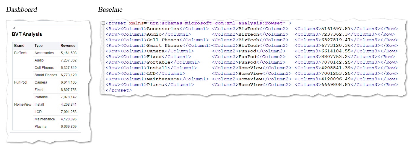
Dashboard looks good, but values in the XML have decimal digits.
As you can see, the analyses are the same or at least they look very similar but the XMLs produced by BVT aren't. From regression point of view this dashboard must get "DASHBOARDS PASSED" result, but it got "DASHBOARDS DIFFERENT".
Reading the documentation gave us no clear explanation for this behaviour. We had to go deeper and understand what actually caused it. Is it BVT screwing up the data it gets from 12c? Well, that is a highly improbable theory. Decimals were not simply present in the result but they were correct. Correct as in "the same as stored in the database", we had to reject this theory.
Or maybe the problem is that BVT works differently with 11g and 12c? Well, this looks more plausible. A few years have passed since 11.1.1.7 was released and it would not be too surprising if the old version and the modern one had different APIs used by BVT and causing this problem. Or maybe the problem is that 12c itself ignores formatting settings. Let's find out.
The Tool
Neither BVT, nor OBIEE logs gave us any insights. From every point of view, everything was working fine. Except that we were getting 100% mismatch between the source and the target. My hypothesis was that BVT worked differently with OBIEE 11g and 12c. How can I check this? Decompiling the tool and reading its code would possibly give me the answer, but it is not legal. And even if it was legal, the latest BVT size is more than 160 megabytes which would give an insane amount of code to read, especially considering the fact I don't actually know what I'm looking for. Not an option. But BVT talks to OBIEE via the network, right? Therefore we can intercept the network traffic and read it. Shall we?
There are a lot of ways to do it. I work with OBIEE quite a lot and Windows is the obvious choice for my platform. And hence the obvious tool for me was Wireshark.
Wireshark is the world’s foremost and widely-used network protocol analyzer. It lets you see what’s happening on your network at a microscopic level and is the de facto (and often de jure) standard across many commercial and non-profit enterprises, government agencies, and educational institutions. Wireshark development thrives thanks to the volunteer contributions of networking experts around the globe and is the continuation of a project started by Gerald Combs in 1998.
What this "About" doesn't say is that Wireshark is open-source and free. Which is quite nice I think.
Installation Details
I'm not going to go into too many details about the installation process. It is quite simple and straightforward. Keep all the defaults unless you know what you are doing, reboot if asked and you are fine.
If you've never used Wireshark or analogues, the main question would be "Where to install it?". The answer is pretty simple - install it on your workstation, the same workstation where BVT is installed. We're going to intercept our own traffic, not someone else's.
A Bit of Wireshark
Before going to the task we want to solve let's spend some time familiarizing with Wireshark. Its starting screen shows all the network adapters I have on my machine. The one I'm using to connect to the OBIEE servers is "WiFi 2".
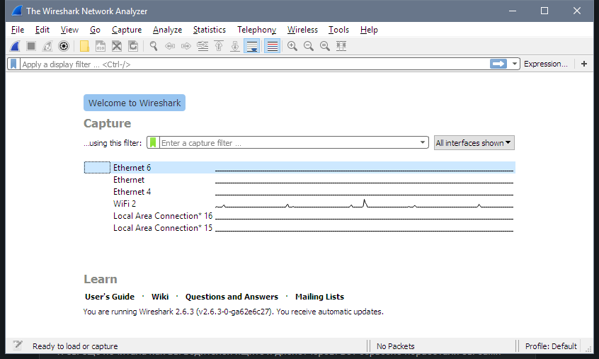
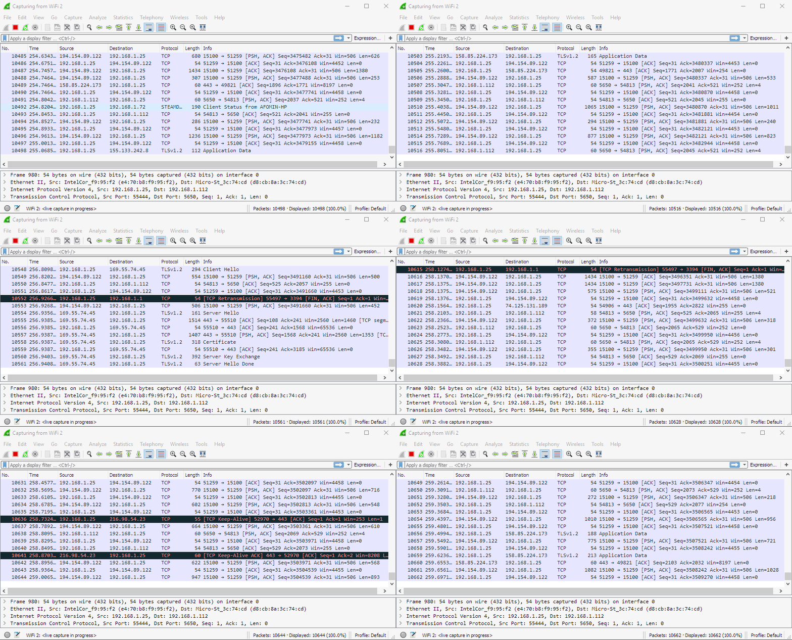
I double-click it and immediately see a constant flow of network packets flying back and forth between my computer and local network machines and the Internet. It's a bit hard to see any particular server in this stream. And "a bit hard" is quite an understatement, to be honest, it is impossible.
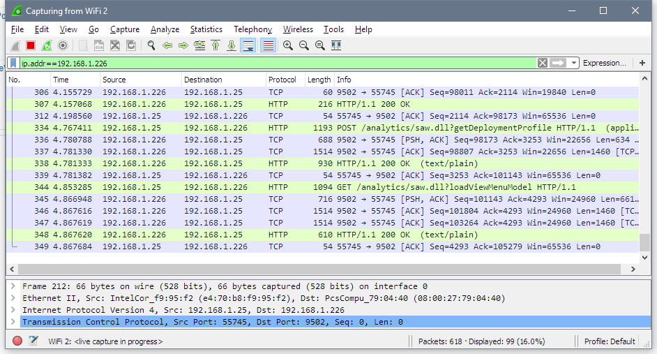
I need a filter. For example, I know that my OBIEE 12c instance IP is 192.168.1.226. So I add ip.addr==192.168.1.226 filter saying that I only want to see traffic to or from this machine. Nothing to see right now, but if I open the login page in a browser, for example, I can see traffic between my machine (192.168.1.25) and the server. It is much better now but still not perfect.
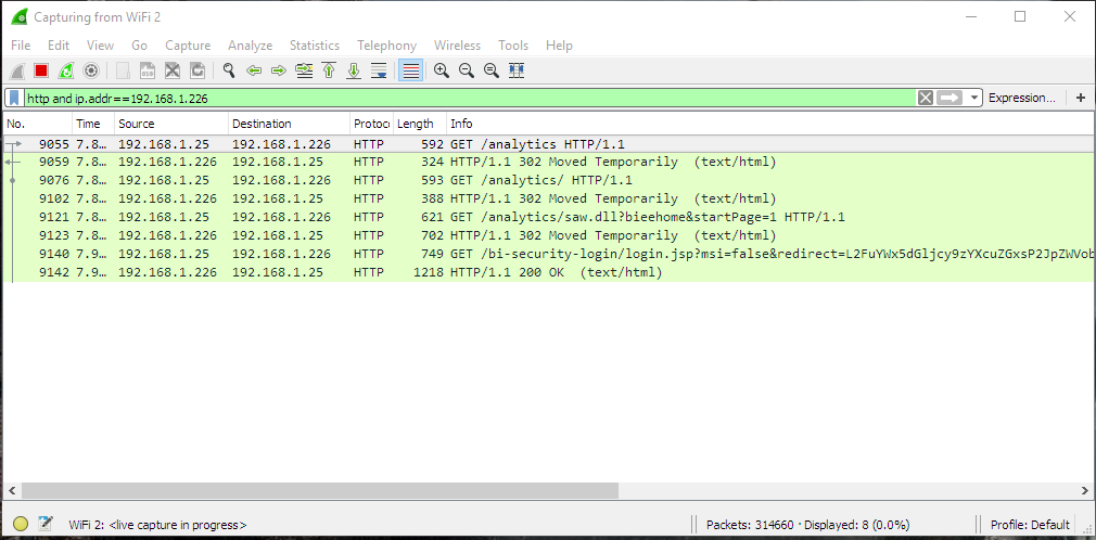
If I add http to the filter like this http and ip.addr==192.168.1.226, I definitely can get a much more clear view.
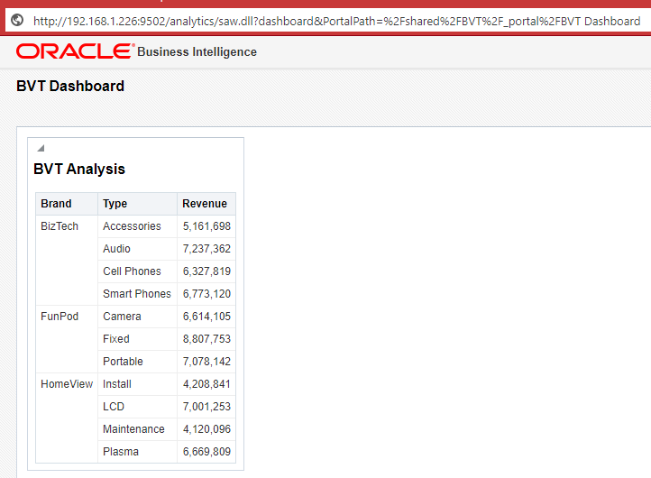
For example, here I opened http://192.168.1.226:9502/analytics page just like any other user would do. There are quite a lot of requests and responses. The browser asked for /analytics URL, the server after a few redirects replied what the actual address for this URL is login.jsp page, then browser requested /bi-security-login/login.jsp page using GET method and got the with HTTP code 200. Code 200 shows that there were no issues with the request.
Let's try to log in.
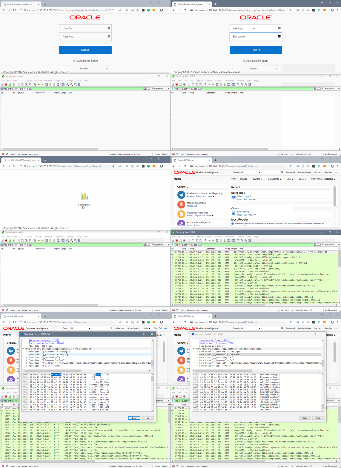
The top window is a normal browser and the bottom one is Wireshark. Note that my credentials been sent via clear text and I think that is a very good argument in defence of using HTTPS everywhere.
That is a very basic use of Wireshark: start monitoring, do something, see what was captured. I barely scratched the surface of what Wireshark can do, but that is enough for my task.
Wireshark and BVT 12c
The idea is quite simple. I should start capturing my traffic then use BVT as usual and see how it works with 12c and then how it works with 11g. This should give me the answer I need.
Let's see how it works with 12c first. To make things more simple I created a catalogue folder with just one analysis placed on a dashboard.
It's time to run BVT and see what happens.

Here is the dataset I got from OBIEE 12c. I slightly edited and formatted it to make easier to read, but didn't change anything important.
What did BVT do to get this result? What API did it use? Let's look at Wireshark.
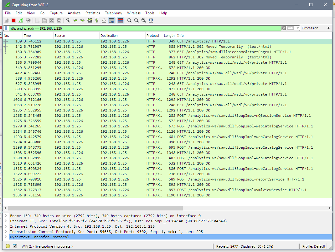
First three lines are the same as with a browser. I don't know why it is needed for BVT, but I don't mind. Then BVT gets WSDL from OBIEE (GET /analytics-ws/saw.dll/wsdl/v6/private). There are multiple pairs of similar query-response flying back and forth because WSDL is big enough and downloaded in chunks. A purely technical thing, nothing strange or important here.
But now we know what API BVT uses to get data from OBIEE. I don't think anyone is surprised that it is Web Services API. Let's take a look at Web Services calls.
First logon method from nQSessionService. It logs into OBIEE and starts a session.
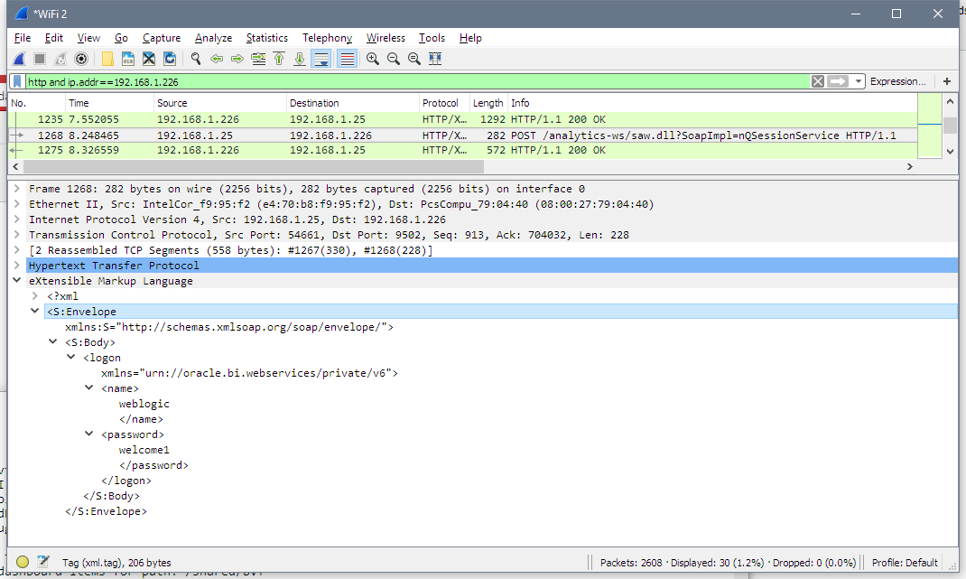
Next requests get catalogue items descriptions for objects in my /shared/BVT folder. We can see a set of calls to webCatalogServce methods. These calls are reading my web catalogue structure: all folders, subfolders, dashboard and analysis. Pretty simple, nothing really interesting or unexpected here.
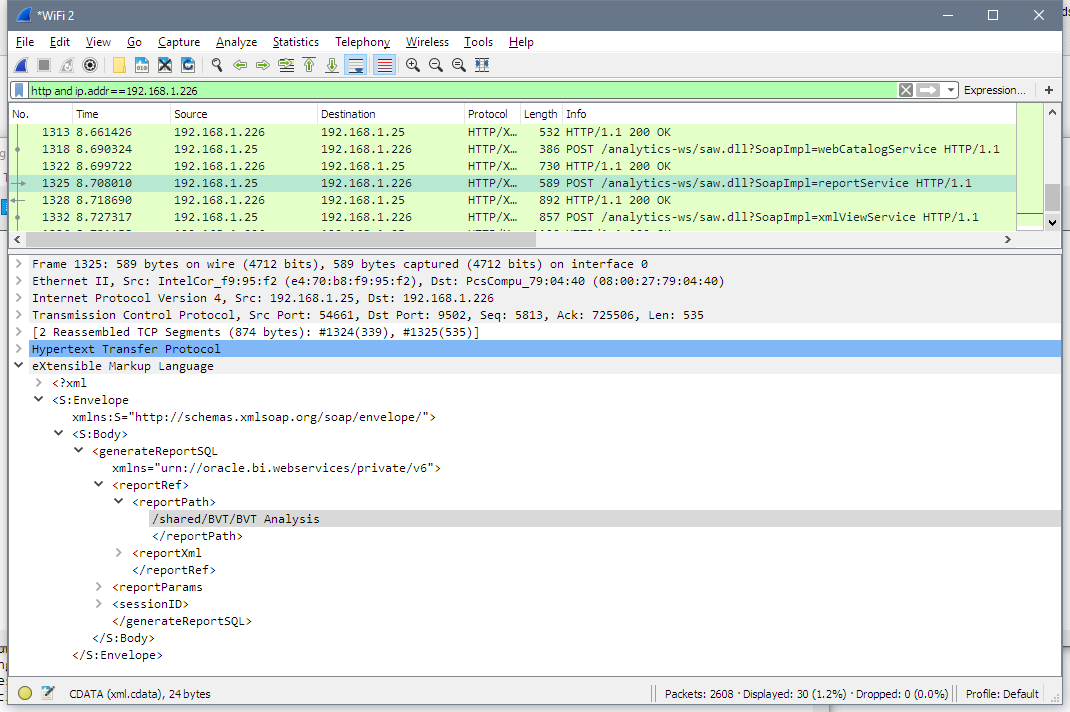
Then we can see how BVT uses generateReportSQLResult from reportService to get logical SQL for the analysis.
And gets analysis' logical SQL as the response.
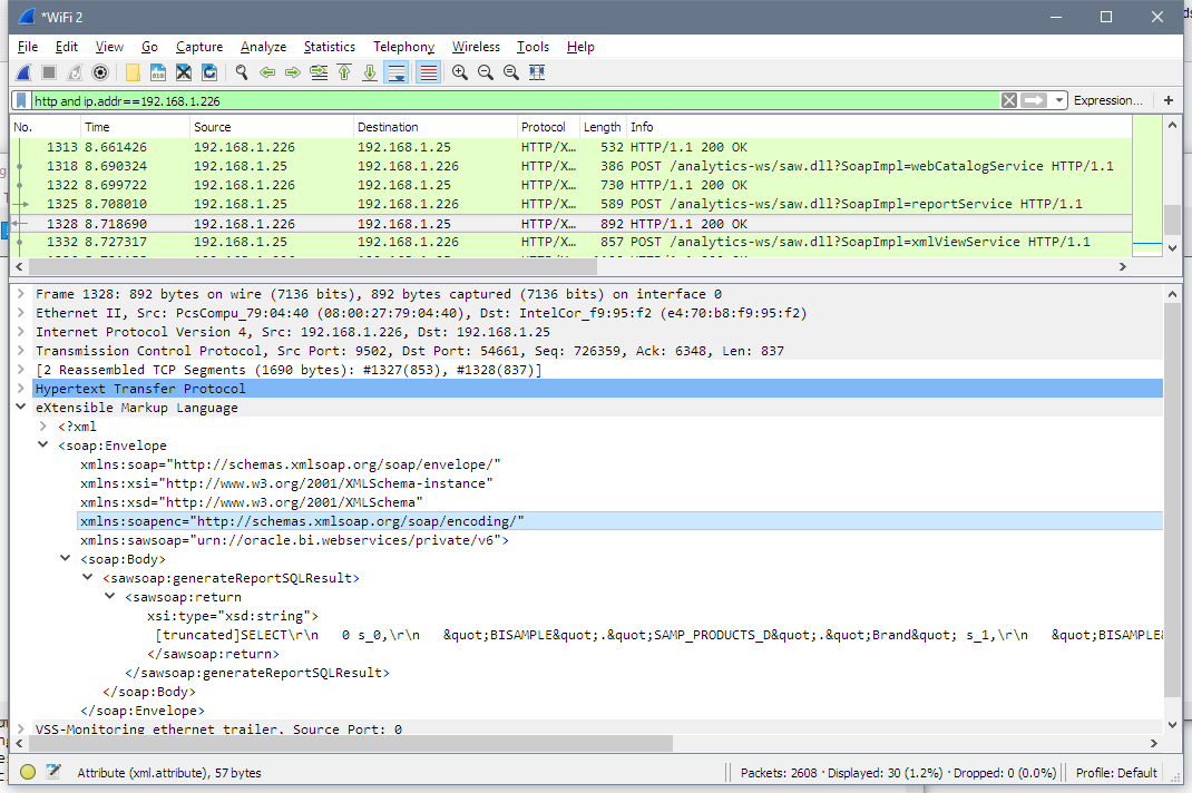
And the final step - BVT executes this SQL and gets the data. Unfortunately, it is hard to show the data on a screenshot, but the line starting with [truncated] is the XML I showed before.
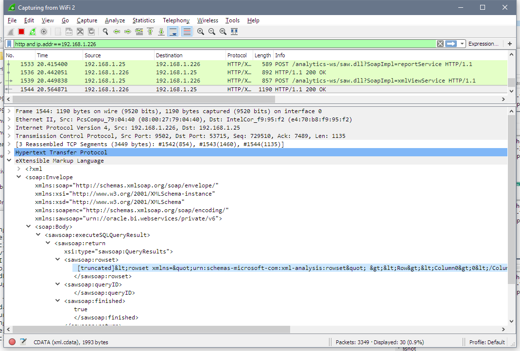
And that's all. That's is how BVT gets data from OBIEE.
I did the same for 11g and saw absolutely the same procedure.
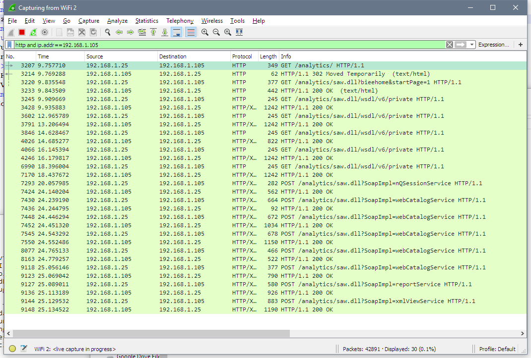
My initial theory that BVT may have been using different APIs for 11g and 12c was busted.
From my experiment, I found out that BVT used xmlViewService to actually get the data. And also I know now that it uses logical SQL for getting the data. Looking at the documentation I can see that xmlViewService has no options related to any formatting. It is a purely data-retrieval service. It can't preserve any formatting and supposed to give only the data. But hey, I've started with the statement "11g preserves formatting", how is that possible? Well, that was a simple coincidence. It doesn't.
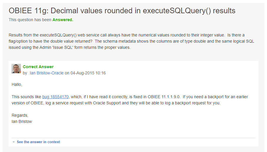
In the beginning, I had very little understanding of what keywords to use on MoS to solve the issue. "BVT for 12c doesn't preserve formatting"? "BVT decimal part settings"? "BVT works differently for 11g and 12c"? Now I have something much better - "executeSQLQuery decimal". 30 seconds of searching and I know the answer.
This was fixed in 11.1.1.9, but there is a patch for 11.1.1.7.some_of_them. The patch fixes an 11g issue which prevents BVT from getting decimal parts of numbers.
As you may have noticed I had no chance of finding this using my initial problem description. Nether BVT, nor 12g or 11.1.1.7 were mentioned. This thread looks completely unrelated to the issue, I had zero chances to find it.
Conlusion
OBIEE is a complex software and solving issues is not always easy. Unfortunately, no single method is enough for solving all problems. Usually, log files will help you. But when something works but not the way you expect, log files can be useless. In my case BVT was working fine, 11g was working fine, 12c was working fine too. Nothing special to write to logs was happening. That is why sometimes you may need unexpected tools. Just like this. Thanks for reading!
Looker for OBIEE Experts: Introduction and Concepts

Recently I've been doing some personal study around various areas including streaming, machine learning and data visualization and one of the tools that got my attention is Looker. I've initially heard about Looker from a Drill to Detail podcast and increasingly been hearing about it in conferences and use cases together with other cloud solutions like BigQuery, Snowflake and Fivetran.
I decided to give it a try myself and, since most of my career was based on Oracle Business Intelligence (OBI) writing down a comparison between the tools that could help others sharing my experience getting introduced to Looker.
OBIEE's Golden Feature: The Semantic Model
As you probably know if you have been working with OBIEE for some time the centrepiece of its architecture is the Semantic Model contained in the Repository (RPD)
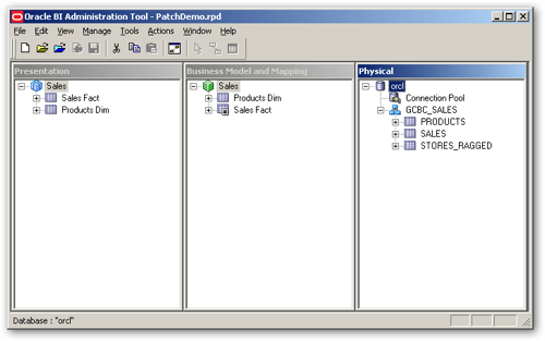
In the three layers of the RPD, we model our source data (e.g. database tables) into attributes, metrics, hierarchies which can then be easily dragged and dropped by the end-user in the analysis or data visualization.
I called the RPD "OBIEE's Golden Feature" because to me it's the main benefit of the platform: abstracting the data complexity from end-users and, at the same time, optimizing the query definition to take care of all the features that could be set in the datasource. The importance of the RPD is also its centrality: within the traditional OBIEE all Analysis and Dashboard had to be based on Subject Areas exposed by the RPD meaning that the definition of the metrics was done in a unique place in a consistent manner and then spread across all the reporting providing the unique source of truth for the important KPIs in the company typical of what Gartner calls the Mode 1 Analytics.
RPD Development Speed Limitation and Mode 2 Analytics
The RPD is a centralized binary object within the OBIEE infrastructure: in order to develop and test a full OBIEE instance is required, and the merges between different streams are natively performed via the RPD's admin tool.
This complexity unified to the deep knowledge required to correctly build a valid semantic model limits the number of people being able to create and publish new content thus slowing down the process from data to insights typical of the centralized Mode 1 Analytic platform provided centrally by IT teams. Moreover, RPD development is entirely point-and-click within the admintool which is somehow considered slow and old fashion in a world of scripting, code versioning and git merging. Several solutions are out in the market (including Rittman Mead Developer Toolkit) to enhance the agility of the development but still, the skills and the toolset required to develop new content makes it a purely IT manageable solution.
In order to overcome this limitation several tools like Tableau, QlikView or Oracle's Data Visualization (included in OAC or in the Desktop version) give all the power in the ends of the end-user: from data-sources to graphing, the tools allow an end-to-end data discovery to visualization journey. The problem with those tools (called Mode 2 Analytics by Gartner) is that there is no central definition of the KPI since it's demanded to every analyst. All those tools are addressing the problem by providing some sort of datasource certification allowing a datasource to be visible and reusable publicly only when it's validated centrally. Again, for most of those tools, the modelling is done in a visual format, which makes it difficult to debug, version control and automate. I've been speaking about this subject in my presentation "DevOps and OBIEE do it before it's too late".
What if we could provide the same centralized source of truth data modelling with an easily scriptable syntax that can be developed from business users without any deep knowledge of SQL or source tables? Well, what we just described is LookML!
LookML
LookerML takes the best part of OBIEE: the idea of a modelling layer and democratizes it in order to be available to all business user with a simple language and set of concepts. Moreover, the code versioning is embedded in the tool, so there's no need to teach git branch, commit, push or pull to non-IT people.
So, what are the concepts behing LookerML and how can you get familiar with it when comparing it to the medatada modelling in the RPD?
LookML Concepts
Let's start from the basic of the RPD modelling: a database table. In LookerML each table is represented by an object called View (naming is a bit confusing). Moreover, LookerML's Views can be used not only to map existing database tables but also to create new tables based on existing content and a SQL definition, like the opaque views in OBIEE. On top of this LookML allows the phisicalization of those objects (into a table) and the definition of a schedule for the refresh. This concept is very useful when aggregates are needed, the aggregate definition (SQL) is defined within the LookML View together with the related refresh schedule.
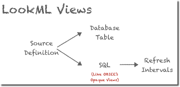
The View itself defines only the source, a bit like the RPD's physical layer, the next step is defining how multiple Views interact within each other, or, in OBIEE terms, the Business Layer. In LookML there is an entity called Explores and is the place where we can define which Views we want to group together, and what's the linkage between them. Multiple Explores are defined in a Model, which should be unique per database. So, in OBIEE words, a Model can be compared to a Business Model with Explores being a subset of Facts and Dimensions grouped in a Subject Area.
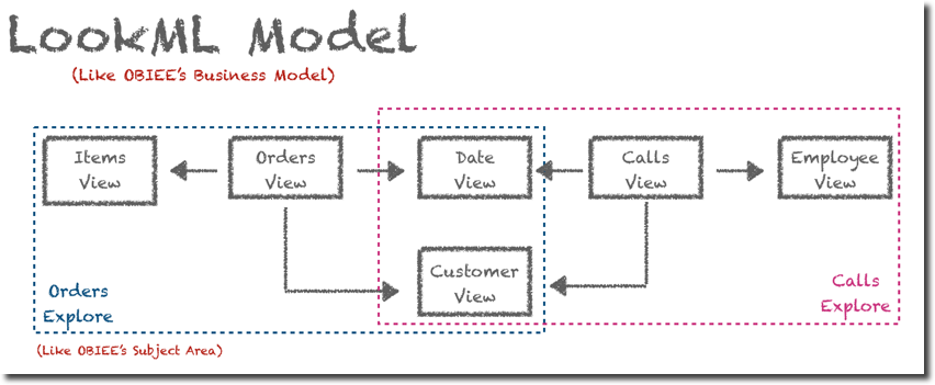
Ok, all "easy" so far, but where do we map the columns? and where do we set the aggregations? As you might expect both are mapped within a LookML View into Fields. Fields is a generic term which includes in both metrics and attributes, LookML naming is the below:
- Dimension: in OBIEE's terms attributes of a dimension. The terminology is confusing since in LookML the Dimension is the column itself while in OBIEE terms is the table. A Dimension can be a column value or a combination of multiple values (like OBIEE's BM Logical Sources formulas). A Dimension in LookML can't have any aggregation (as in OBIEE).
- Measures: in OBIEE's terms a metric. The definition includes, the source formula in SQL syntax, the type of aggregation (min/max/count...) and the drill fields.
Filters: this is not something usually defined in OBIEE's RPD, filters are a way of passing a user choice based on a column value back to an RPD calculation formula, a bit like, for the OBIEE experts, overriding session variables with dashboard prompt values. - Parameters: again this is not something usually defined in OBIEE's RPD, you can think a Parameter as a way of setting up variables function. E.g. a Parameter with values SUM, AVG, MIN, MAX could be used to change how a certain Measure is aggregated
All good so far? Stick with me and in the future we'll explore more about LookML syntax and Looker in general!
Parsing Badly Formatted JSON in Oracle DB with APEX_JSON

After some blogging silence due to project work and holidays, I thought it was a good idea to do a write-up about a problem I faced this week. One of the tasks I was assigned was to parse a set of JSON files stored in an Oracle 12.1 DB Table.
As probably all of you already know JSON (JavaScript Object Notation) is a lightweight data-interchange format and is the format used widely when talking of web-services due to its flexibility. In JSON there is no header to define (think CSV as example), every field is defined in a format like "field name":"field value", there is no "set of required columns" for a JSON object, when a new attribute needs to be defined, the related name and value can be added to the structure. On top of this "schema-free" definition, the field value can either be
- a single value
- an array
- a nested JSON object
Basically, when you start parsing JSON you feel like

The Easy Part
The task assigned wasn't too difficult, after reading the proper documentation, I was able to parse a JSON File like
{
 "field1": "abc",
 "field2": "cde"
}
Using a simple SQL like
select *
 from TBL_NAME d,
 JSON_TABLE(d.text, '$' COLUMNS (
   field1 VARCHAR2(10) PATH '$.field1',
   field2 VARCHAR2(10) PATH '$.field2'
   )
 )
Parsing arrays is not very complex either, a JSON file like
{
 "field1": "abc",
 "field2": "cde",
 "field3": ["fgh","ilm","nop"]
}
Can be easily parsed using the NESTED PATH call
select *
 from TBL_NAME d,
 JSON_TABLE(d.text, '$' COLUMNS (
   field1 VARCHAR2(10) PATH '$.field1',
   field2 VARCHAR2(10) PATH '$.field2',
   NESTED PATH '$.field3[*]' COLUMNS (
     field3 VARCHAR2(10) PATH '$'
   )
 )
)
In case the Array contains nested objects, those can be parsed using the same syntax as before, for example, field4 and field5 of the following JSON
{
 "field1": "abc",
 "field2": "cde",
 "field3": [
           {
            "field4":"fgh",
            "field5":"ilm"
           },
           {
            "field4":"nop",
            "field5":"qrs"
           }
           ]
}
can be parsed with
NESTED PATH '$.field3[*]' COLUMNS (
   field4 VARCHAR2(10) PATH '$.field4',
   field5 VARCHAR2(10) PATH '$.field5'
)
...Where things got complicated
All very very easy with well-formatted JSON files, but then I faced the following
{
"field1": "abc",
"field2": "cde",
"field3": [
    {
     "field4": "aaaa",
     "field5":{
           "1234":"8881",
           "5678":"8893"
          }
     },
     {
      "field4": "bbbb",
      "field5":{
            "9876":"8881",
            "7654":"8945",
            "4356":"7777"
          }
      }
      ]
}
Basically the JSON file started including fields with names representing the Ids meaning an association like Product Id (1234) is member of Brand Id (8881). This immediately triggered my reaction:

After checking the documentation again, I wasn't able to find anything that could help me parsing that, since all the calls were including a predefined PATH string, that in the case of Ids I couldn't know beforehand.
I then reached out to my network on Twitter
To all my @Oracle SQL friends out there: I need to parse a JSON object which has a strange format of {“name”:”abc”, “345678”:”123456”} with the 345678 being an Id I need to extract, any suggestions? none of the ones mentioned here seems to help https://t.co/DRWdGvCVfu pic.twitter.com/PfhtUnAeR4
— Francesco Tisiot (@FTisiot) 14 agosto 2018
That generated quite a lot of responses. Initially, the discussion was related to the correctness of the JSON structure, that, from a purist point of view should be mapped as
{
"field1": "abc",
"field2": "cde",
"field3": [
     {
      "field4": "aaaa",
      "field5":
           {
             "association": [
                  {"productId":"1234", "brandId":"8881"},
                  {"productId":"5678", "brandId":"8893"}
                  ]
           },
      },
      {
       "field4": "bbbb",
       "field5":
           {
             "association": [
                  {"productId":"9876", "brandId":"8881"},
                  {"productId":"7654", "brandId":"8945"},
                  {"productId":"4356", "brandId":"7777"}
                  ]
           }
      }
      ]
}
basically going back to standard field names like productId and brandId that could be easily parsed. In my case this wasn't possible since the JSON format was aready widely used at the client.
Possible Solutions
Since a change in the JSON format wasn't possible, I needed to find a way of parsing it, few solutions were mentioned in the twitter thread:
- Regular Expressions
- Bash external table preprocessor
- Java Stored functions
- External parsing before storing data into the database
All the above were somehow discarded since I wanted to try achieving a solution based only on existing database functions. Other suggestion included JSON_DATAGUIDE and JSON_OBJECT.GET_KEYS that unfortunately are available only from 12.2 (I was on 12.1).
But, just a second before surrendering, Alan Arentsen suggested using APEX_JSON.PARSE procedure!
The Chosen One: APEX_JSON
The APEX_JSON package offers a series of procedures to parse JSON in a PL/SQL package, in particular:
- PARSE: Parses a JSON formatted string contained in a
VARCHAR2orCLOBstoring all the members. - GET_COUNT: Returns the number of array elements or object members
- GET_MEMBERS: Returns the table of members of an object
You can already imagine how a combination of those calls can parse the JSON text defined above, let's have a look at the JSON again:
{
"field1": "abc",
"field2": "cde",
"field3": [
    {
     "field4": "aaaa",
     "field5":{
           "1234":"8881",
           "5678":"8893"
          }
     },
     {
      "field4": "bbbb",
      "field5":{
            "9876":"8881",
            "7654":"8945",
            "4356":"7777"
          }
      }
      ]
}
The parsing process should iterate over the field3 entries (2 in this case), and for each entry, then iterate over the fields in field5 to get both the field name as well as the field value.
The number of field3 entries can be found with
APEX_JSON.GET_COUNT(p_path=>'field3',p_values=>j);
And the list of members of field5 with
APEX_JSON.GET_MEMBERS(p_path=>'field3[%d].field5',p_values=>j,p0=>i);
Note the p_path parameter set to field3[%d].field5 meaning that we want to extract the field5 from the nth row in field3. The rownumber is defined by p0=>i with i being the variable we use in our FOR loop.
The complete code is the following
DECLARE
   j APEX_JSON.t_values;
   r_count number;
   field5members   WWV_FLOW_T_VARCHAR2;
   p0 number;
   BrandId VARCHAR2(10);
BEGIN
APEX_JSON.parse(j,'<INSERT_JSON_STRING>');
# Getting number of field3 elements
r_count := APEX_JSON.GET_COUNT(p_path=>'field3',p_values=>j);
dbms_output.put_line('Nr Records: ' || r_count);

# Looping for each element in field3
FOR i IN 1 .. r_count LOOP
# Getting field5 members for the ith member of field3
 field5members := APEX_JSON.GET_MEMBERS(p_path=>'field3[%d].field5',p_values=>j,p0=>i);
# Looping all field5 members
 FOR q in 1 .. field5members.COUNT LOOP
# Extracting BrandId
   BrandId := APEX_JSON.GET_VARCHAR2(p_path=>'field3[%d].field5.'||field5members(q) ,p_values=>j,p0=>i);
# Printing BrandId and Product Id
   dbms_output.put_line('Product Id ="'||field5members(q)||'" BrandId="'||BrandId ||'"');
 END LOOP;
END LOOP;

END;
Note that, in order to extract the BrandId we used
APEX_JSON.GET_VARCHAR2(p_path=>'field3[%d].field5.'||field5members(q) ,p_values=>j,p0=>i);
Specifically the PATH is field3[%d].field5.'||field5members(q). As you can imagine we are appending the member name (field5members(q)) to the path described previously to extract the value, forming a string like field3[1].field5.1234 that will correctly extract the value associated.
Conclusion
Three things to save from this experience. The first is the usage of JSON_TABLE: with JSON_TABLE you can parse well-constructed JSON documents and it's very easy and powerful.
The second: APEX_JSON useful package to parse "not very well" constructed JSON documents, allows iteration across elements of JSON arrays and object members.
The last, which is becoming every day more relevant in my career, is the importance of networking and knowledge sharing: blogging, speaking at conferences, helping others in various channels allows you to know other people and be known with the nice side effect of sometimes being able with a single tweet to get help solving problems you may face!
Making our way into Dremio
In an analytics system, we typically have an Operational Data Store (ODS) or staging layer; a performance layer or some data marts; and on top, there would be an exploration or reporting tool such as Tableau or Oracle's OBIEE. This architecture can lead to latency in decision making, creating a gap between analysis and action. Data preparation tools like Dremio can address this.
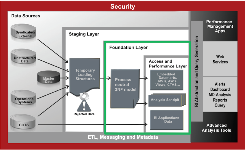
Dremio is a Data-as-a-Service platform allowing users to quickly query data, directly from the source or in any layer, regardless of its size or structure. The product makes use of Apache Arrow, allowing it to virtualise data through an in-memory layer, creating what is called a Data Reflection.
The intent of this post is an introduction to Dremio; it provides a step by step guide on how to query data from Amazon's S3 platform.
I wrote this post using my MacBook Pro, Dremio is supported on MacOS. To install it, I needed to make some configuration changes due to the Java version. The latest version of Dremio uses Java 1.8. If you have a more recent Java version installed, you’ll need to make some adjustments to the Dremio configuration files.
Lets start downloading Dremio and installing it. Dremio can be found for multiple platforms and we can download it from here.
Dremio uses Java 1.8, so if you have an early version please make sure you install java 1.8 and edit /Applications/Dremio.app/Contents/Java/dremio/conf/dremio-env to point to the directory where java 1.8 home is located.

After that you should be able to start Dremio as any other MacOs application and access http://localhost:9047
Configuring S3 Source
Dremio can connect to relational databases (both commercial and open source), NoSQL, Hadoop, cloud storage, ElasticSearch, among others. However the scope of this post is to use a well known NoSQL storage S3 bucket (more details can be found here) and show the query capabilities of Dremio against unstructured data.
For this demo we're using Garmin CSV activity data that can be easily downloaded from Garmin activity page.
Here and example of a CSV Garmin activity. If you don't have a Garmin account you can always replicate the data above.
act,runner,Split,Time,Moving Time,Distance,Elevation Gain,Elev Loss,Avg Pace,Avg Moving Paces,Best Pace,Avg Run Cadence,Max Run Cadence,Avg Stride Length,Avg HR,Max HR,Avg Temperature,Calories
1,NMG,1,00:06:08.258,00:06:06.00,1,36,--,0:06:08  ,0:06:06  ,0:04:13  ,175.390625,193.0,92.89507499768523,--,--,--,65
1,NMG,2,00:10:26.907,00:10:09.00,1,129,--,0:10:26  ,0:10:08  ,0:06:02  ,150.140625,236.0,63.74555754497759,--,--,--,55
For user information data we have used the following dataset
runner,dob,name
JM,01-01-1900,Jon Mead
NMG,01-01-1900,Nelio Guimaraes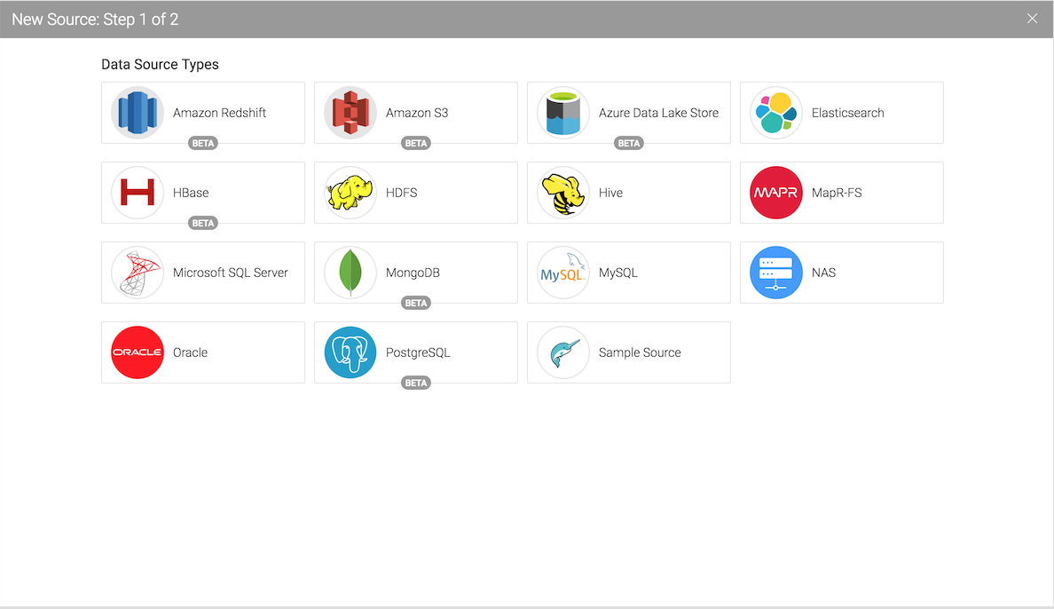
Add your S3 credentials to access
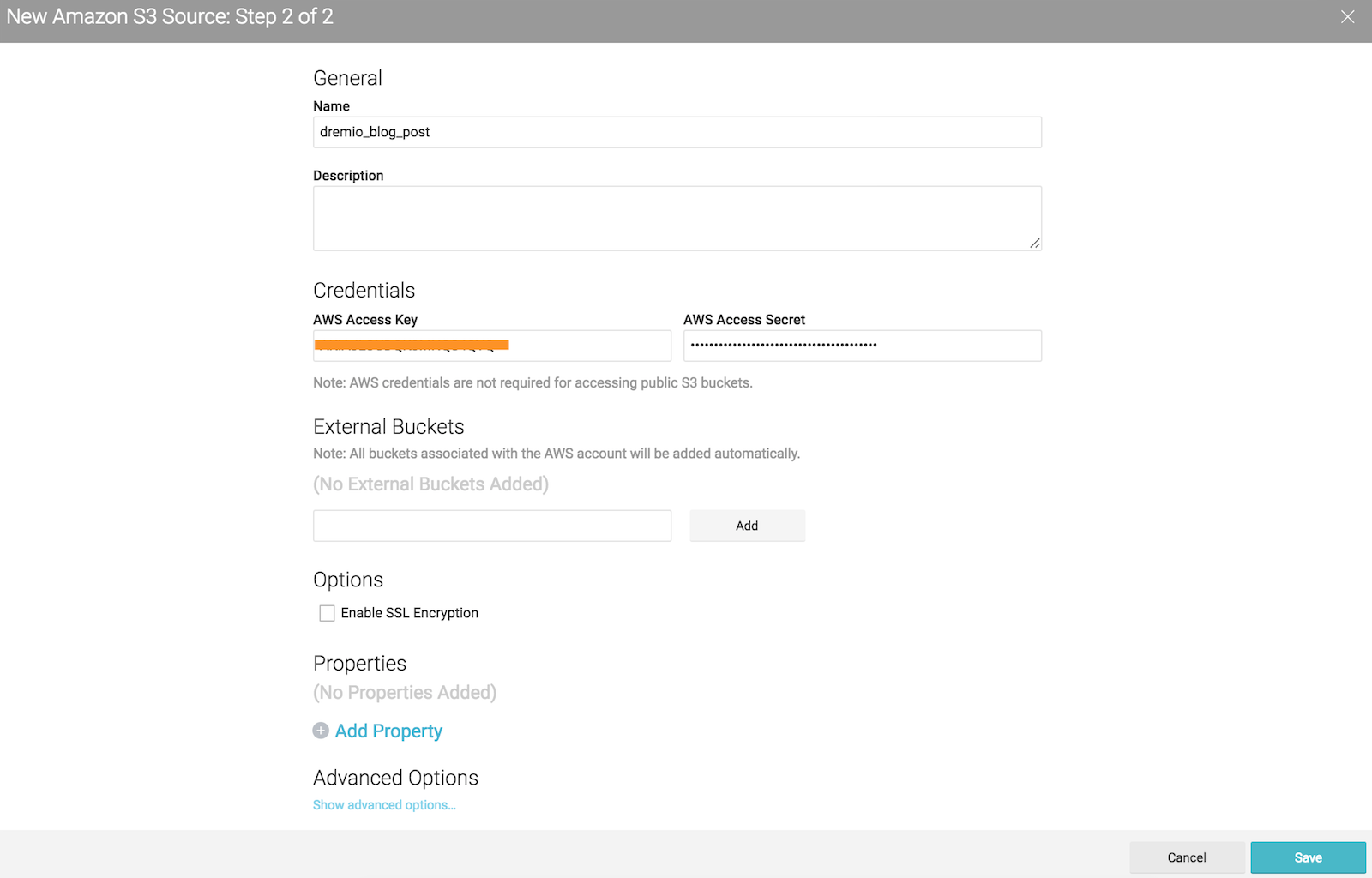
After configuring your S3 account all buckets associated to it, will be prompted under the new source area.

For this post I’ve created two buckets : nmgbuckettest and nmgdremiouser containing data that could be interpreted as a data mart
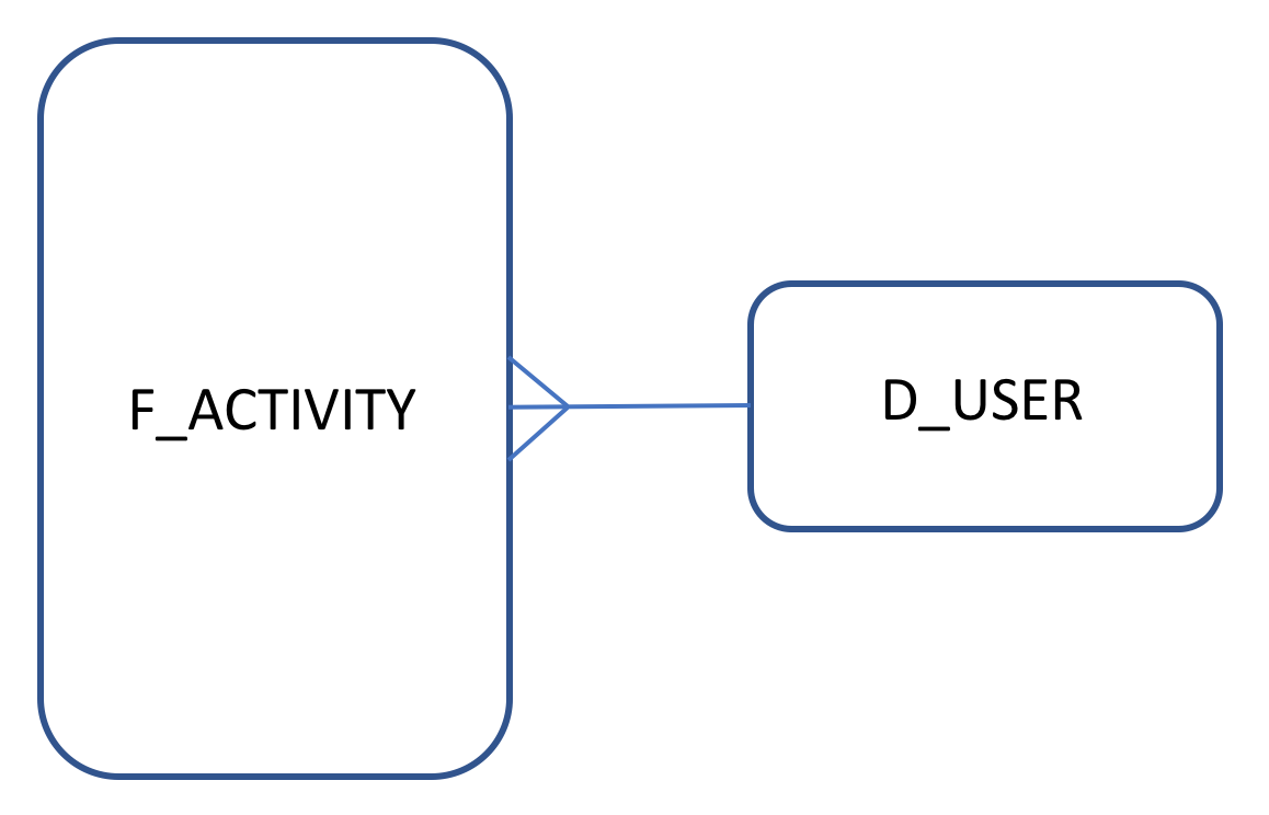
nmgbuckettest - contains Garmin activity data that could be seen as a fact table in CSV format :
Act,Runner,Split,Time,Moving Time,Distance,Elevation Gain,Elev Loss,Avg Pace,Avg Moving Paces,Best Pace,Avg Run Cadence,Max Run Cadence,Avg Stride Length,Avg HR,Max HR,Avg Temperature,Calories
nmgdremiouser - contains user data that could be seen as a user dimension in a CSV format:
runner,dob,name
Creating datasets
After we add the S3 buckets we need to set up the CSV format. Dremio makes most of the work for us, however we had the need to adjust some fields, for example date formats or map a field as an integer.

By clicking on the gear icon we access the following a configuration panel where we can set the following options. Our CSV's were pretty clean so I've just change the line delimiter for \n and checked the option Extract Field Name
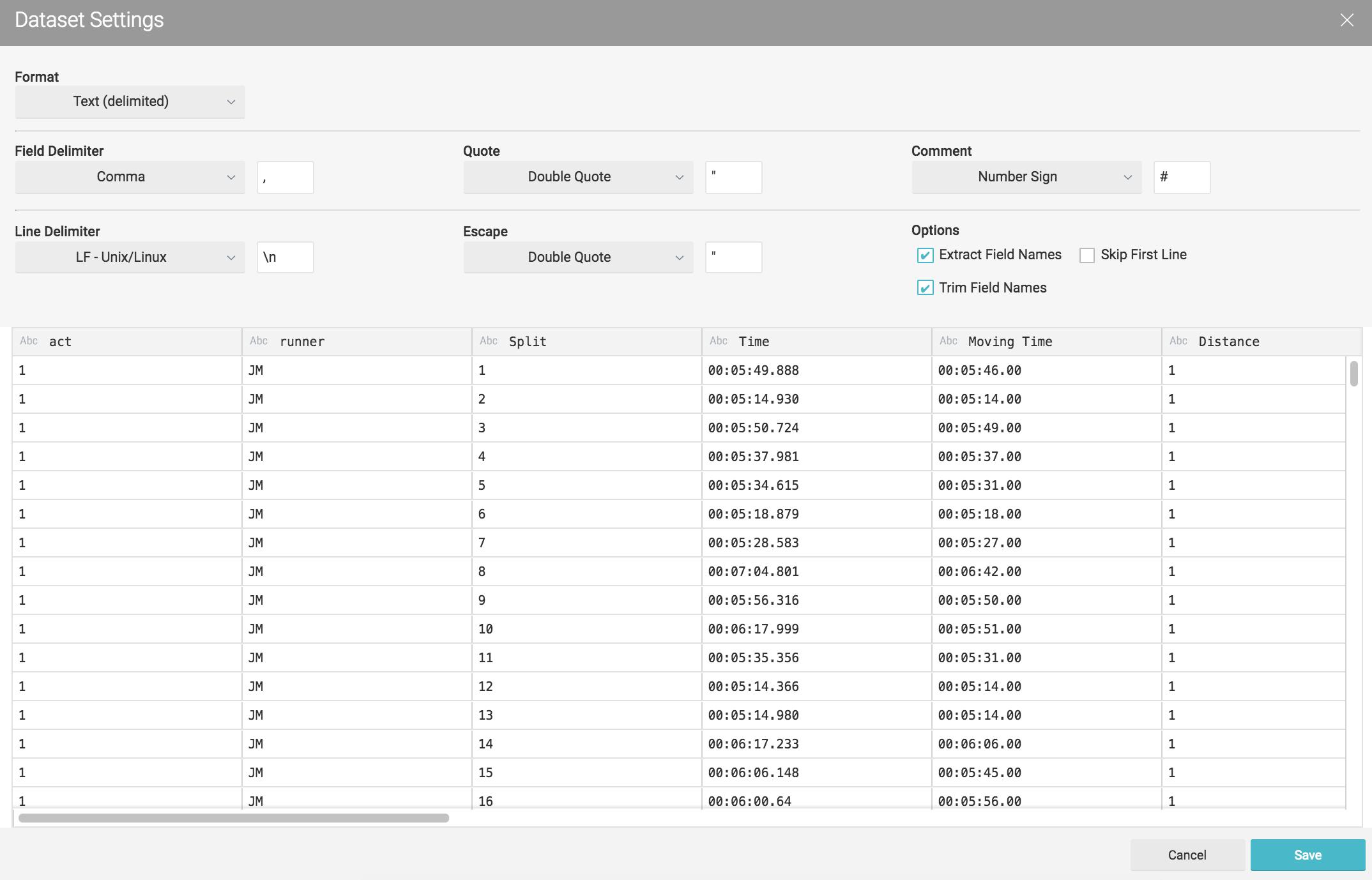
Lets do the same for the second set of CSV's (nmgdremiouser bucket)
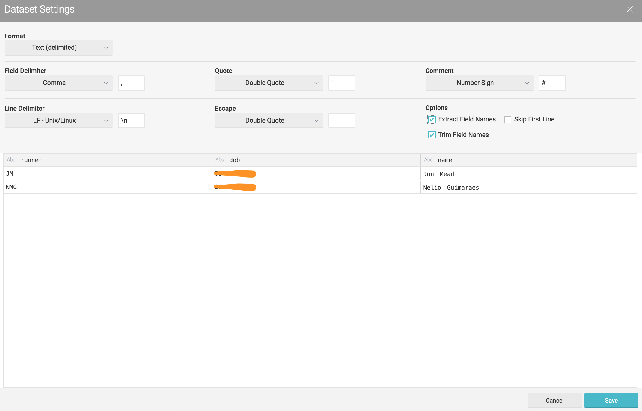
Click in saving will drive us to a new panel where we can start performing some queries.

However as mentioned before at this stage we might want to adjust some fields. Right here I'll adapt the dob field from the nmgdremiouser bucket to be in the dd-mm-yyyy format.
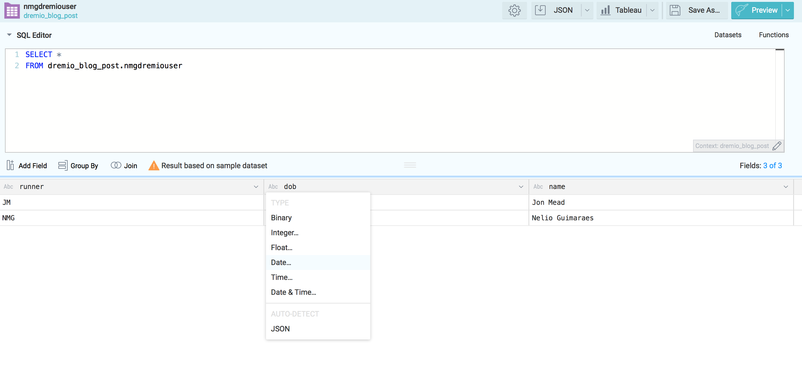
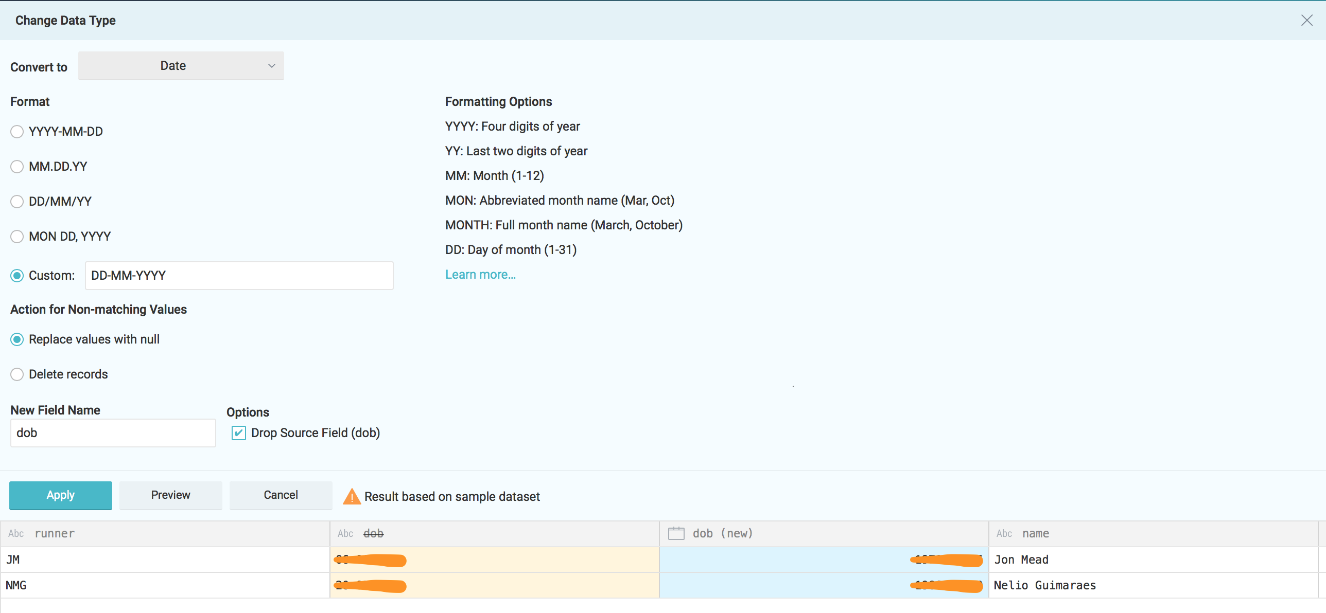
Apply the changes and save the new dataset under the desire space.
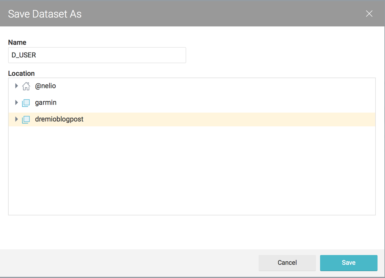
Feel free to do the same for the nmgbuckettest CSV's. As part of my plan to make I'll call D_USER for the dataset coming from nmgdremiouser bucket and F_ACTIVITY for data coming from nmgbuckettest

Querying datasets
Now that we have DUSER and FACTIVITY datasets created we can start querying them and do some analysis.
This first analysis will tell us which runner climbs more during his activities:
SELECT round(nested_0.avg_elev_gain) AS avg_elev_gain, round(nested_0.max_elev_gain) AS max_elev_gain, round(nested_0.sum_elev_gain) as sum_elev_gain, join_D_USER.name AS name
FROM (
  SELECT avg_elev_gain, max_elev_gain, sum_elev_gain, runner
  FROM (
    SELECT AVG(to_number("Elevation Gain",'###')) as avg_elev_gain,
    MAX(to_number("Elevation Gain",'###')) as max_elev_gain,
    SUM(to_number("Elevation Gain",'###')) as sum_elev_gain,
    runner
    FROM dremioblogpost.F_ACTIVITY
    where "Elevation Gain" != '--'
    group by runner
  ) nested_0
) nested_0
INNER JOIN dremioblogpost.D_USER AS join_D_USER ON nested_0.runner = join_D_USER.runner 
To enrich the example lets understand who is the fastest runner with analysis based on the total climbing
 SELECT round(nested_0.km_per_hour) AS avg_speed_km_per_hour, nested_0.total_climbing AS total_climbing_in_meters, join_D_USER.name AS name
FROM (
  SELECT km_per_hour, total_climbing, runner
  FROM (
    select avg(cast(3600.0/((cast(substr("Avg Moving Paces",3,2) as integer)*60)+cast(substr("Avg Moving Paces",6,2) as integer)) as float)) as km_per_hour,
        sum(cast("Elevation Gain" as integer)) total_climbing,
        runner
        from dremioblogpost.F_ACTIVITY
        where "Avg Moving Paces" != '--'
        and "Elevation Gain" != '--'
        group by runner
  ) nested_0
) nested_0
 INNER JOIN dremioblogpost.D_USER AS join_D_USER ON nested_0.runner = join_D_USER.runner
Conclusions
Dremio is an interesting tool capable of unifying existing repositories of unstructured data. Is Dremio capable of working with any volume of data and complex relationships? Well, I believe that right now the tool isn't capable of this, even with the simple and small data sets used in this example the performance was not great.
Dremio does successfully provide self service access to most platforms meaning that users don't have to move data around before being able to perform any analysis. This is probably the most exciting part of Dremio. It might well be in the paradigm of a "good enough" way to access data across multiple sources. This will allow data scientists to do analysis before the data is formally structured.
Making our way into Dremio
In an analytics system, we typically have an Operational Data Store (ODS) or staging layer; a performance layer or some data marts; and on top, there would be an exploration or reporting tool such as Tableau or Oracle's OBIEE. This architecture can lead to latency in decision making, creating a gap between analysis and action. Data preparation tools like Dremio can address this.

Dremio is a Data-as-a-Service platform allowing users to quickly query data, directly from the source or in any layer, regardless of its size or structure. The product makes use of Apache Arrow, allowing it to virtualise data through an in-memory layer, creating what is called a Data Reflection.
The intent of this post is an introduction to Dremio; it provides a step by step guide on how to query data from Amazon's S3 platform.
I wrote this post using my MacBook Pro, Dremio is supported on MacOS. To install it, I needed to make some configuration changes due to the Java version. The latest version of Dremio uses Java 1.8. If you have a more recent Java version installed, you’ll need to make some adjustments to the Dremio configuration files.
Lets start downloading Dremio and installing it. Dremio can be found for multiple platforms and we can download it from here.
Dremio uses Java 1.8, so if you have an early version please make sure you install java 1.8 and edit /Applications/Dremio.app/Contents/Java/dremio/conf/dremio-env to point to the directory where java 1.8 home is located.

After that you should be able to start Dremio as any other MacOs application and access http://localhost:9047


Configuring S3 Source
Dremio can connect to relational databases (both commercial and open source), NoSQL, Hadoop, cloud storage, ElasticSearch, among others. However the scope of this post is to use a well known NoSQL storage S3 bucket (more details can be found here) and show the query capabilities of Dremio against unstructured data.
For this demo we're using Garmin CSV activity data that can be easily downloaded from Garmin activity page.
Here and example of a CSV Garmin activity. If you don't have a Garmin account you can always replicate the data above.
act,runner,Split,Time,Moving Time,Distance,Elevation Gain,Elev Loss,Avg Pace,Avg Moving Paces,Best Pace,Avg Run Cadence,Max Run Cadence,Avg Stride Length,Avg HR,Max HR,Avg Temperature,Calories
1,NMG,1,00:06:08.258,00:06:06.00,1,36,--,0:06:08  ,0:06:06  ,0:04:13  ,175.390625,193.0,92.89507499768523,--,--,--,65
1,NMG,2,00:10:26.907,00:10:09.00,1,129,--,0:10:26  ,0:10:08  ,0:06:02  ,150.140625,236.0,63.74555754497759,--,--,--,55
For user information data we have used the following dataset
runner,dob,name
JM,01-01-1900,Jon Mead
NMG,01-01-1900,Nelio Guimaraes
Add your S3 credentials to access

After configuring your S3 account all buckets associated to it, will be prompted under the new source area.

For this post I’ve created two buckets : nmgbuckettest and nmgdremiouser containing data that could be interpreted as a data mart

nmgbuckettest - contains Garmin activity data that could be seen as a fact table in CSV format :
Act,Runner,Split,Time,Moving Time,Distance,Elevation Gain,Elev Loss,Avg Pace,Avg Moving Paces,Best Pace,Avg Run Cadence,Max Run Cadence,Avg Stride Length,Avg HR,Max HR,Avg Temperature,Calories
nmgdremiouser - contains user data that could be seen as a user dimension in a CSV format:
runner,dob,name
Creating datasets
After we add the S3 buckets we need to set up the CSV format. Dremio makes most of the work for us, however we had the need to adjust some fields, for example date formats or map a field as an integer.

By clicking on the gear icon we access the following a configuration panel where we can set the following options. Our CSV's were pretty clean so I've just change the line delimiter for \n and checked the option Extract Field Name

Lets do the same for the second set of CSV's (nmgdremiouser bucket)

Click in saving will drive us to a new panel where we can start performing some queries.

However as mentioned before at this stage we might want to adjust some fields. Right here I'll adapt the dob field from the nmgdremiouser bucket to be in the dd-mm-yyyy format.


Apply the changes and save the new dataset under the desire space.

Feel free to do the same for the nmgbuckettest CSV's. As part of my plan to make I'll call D_USER for the dataset coming from nmgdremiouser bucket and F_ACTIVITY for data coming from nmgbuckettest

Querying datasets
Now that we have D_USER and F_ACTIVITY datasets created we can start querying them and do some analysis.
This first analysis will tell us which runner climbs more during his activities:
SELECT round(nested_0.avg_elev_gain) AS avg_elev_gain, round(nested_0.max_elev_gain) AS max_elev_gain, round(nested_0.sum_elev_gain) as sum_elev_gain, join_D_USER.name AS name
FROM (
  SELECT avg_elev_gain, max_elev_gain, sum_elev_gain, runner
  FROM (
    SELECT AVG(to_number("Elevation Gain",'###')) as avg_elev_gain,
    MAX(to_number("Elevation Gain",'###')) as max_elev_gain,
    SUM(to_number("Elevation Gain",'###')) as sum_elev_gain,
    runner
    FROM dremioblogpost.F_ACTIVITY
    where "Elevation Gain" != '--'
    group by runner
  ) nested_0
) nested_0
INNER JOIN dremioblogpost.D_USER AS join_D_USER ON nested_0.runner = join_D_USER.runner 
To enrich the example lets understand who is the fastest runner with analysis based on the total climbing
 SELECT round(nested_0.km_per_hour) AS avg_speed_km_per_hour, nested_0.total_climbing AS total_climbing_in_meters, join_D_USER.name AS name
FROM (
  SELECT km_per_hour, total_climbing, runner
  FROM (
    select avg(cast(3600.0/((cast(substr("Avg Moving Paces",3,2) as integer)*60)+cast(substr("Avg Moving Paces",6,2) as integer)) as float)) as km_per_hour,
        sum(cast("Elevation Gain" as integer)) total_climbing,
        runner
        from dremioblogpost.F_ACTIVITY
        where "Avg Moving Paces" != '--'
        and "Elevation Gain" != '--'
        group by runner
  ) nested_0
) nested_0
 INNER JOIN dremioblogpost.D_USER AS join_D_USER ON nested_0.runner = join_D_USER.runner
Conclusions
Dremio is an interesting tool capable of unifying existing repositories of unstructured data. Is Dremio capable of working with any volume of data and complex relationships? Well, I believe that right now the tool isn't capable of this, even with the simple and small data sets used in this example the performance was not great.
Dremio does successfully provide self service access to most platforms meaning that users don't have to move data around before being able to perform any analysis. This is probably the most exciting part of Dremio. It might well be in the paradigm of a "good enough" way to access data across multiple sources. This will allow data scientists to do analysis before the data is formally structured.


