Category Archives: Rittman Mead
Where is My Money Going? Checking the balance with Oracle Cloud Account Metering REST APIs

How much did I spend so far?

It's a typical question we ask ourselves daily and what do we do? Probably check the bank account status on our phone and yell at ourselves for all the money we trashed the previous night at the pub.
The Cloud
One of the great benefits of the cloud is that there is no big upfront cost required to start playing with the latest tool or technology, we just need to fill in a few forms, write down the credit card details and there we go! However, the cloud doesn't mean free: most of the times we pay based on resource and time consumption and things can become pretty expensive if we don't manage our resources wisely.
The main Oracle Cloud Dashboard offers a preview of the Month to Date Cost and by clicking on it, we can easily understand the cost per product. Like in the example below we spend £322.8 month to date and precisely £262.80 on Oracle Analytics Classic.
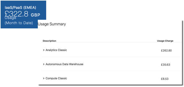
We can go another step down the line: if for example, we have multiple versions of the same product, we'll see a line for each version or licensing method. In our case, all the money comes from a single B88303 - OAC Enterprise Edition OCPU per Hour product with an overall 60 hours of uptime (OAC billing is per hour).

However, this requires a manual login into the Oracle Cloud to check the balance, which is not optimal if we want to display this information in external tools or automate part of the cost-checking procedures. Fortunately, we can retrieve the same information with Oracle Cloud Account Metering REST APIs.
Oracle Cloud Account Metering REST APIs
Oracle Cloud Account Metering REST APIs expose a lot of useful information about our Oracle Cloud account via REST APIs. We can, for example, check our subscription details, credit promotions, resource usage, cost and quotas. All we need to test the REST APIs is cURL, a command-line utility for sending HTTP requests. The syntax to retrieve the data is
curl -X GET -u <USERNAME>:<PASSWORD> \
	-H "X-ID-TENANT-NAME:<TENANT_ID>" \
	"https://itra.oraclecloud.com/<BASE_PATH>/<RESOURCE_NAME>
Where
<USERNAME>and<PASSWORD>are the credentials of an account associated with at least one of the following roles- Identity Domain Administrator
- Cloud Account Administrator
- Service Administrator
<TENANT_ID>is the identity domain ID, you can find it under the Oracle Analytics Cloud -> Overview

<BASE_PATH>is the base URI of the resource, e.g./metering/api/v1<RESOURCE_NAME>is the name of the specific resource we are requesting
Checking the Cost
If, as per the example below, we want to understand the cost, we simply need to call the usagecost resource passing the <ACCOUNT_ID> parameter which can be found in the Overview page of every service we already have in our account.
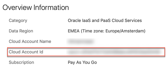
The basic cURL command to check the cost then becomes the following
curl -X GET -u <USERNAME>:<PASSWORD> \
	-H "X-ID-TENANT-NAME:<TENANT_ID>" \
	"https://itra.oraclecloud.com/metering/api/v1/usagecost/<ACCOUNT_ID>?startTime=<START_TIME>&endTime=<ENDTIME>&timeZone=<TIMEZONE>"
Where on top of the parameters defined above we have
<START_TIME>and<END_TIME>with the formatYYYY-MM-DDTHH:mm:sssZe.g.2019-08-01T00:00:00.000<TIMEZONE>we specify which timezone to use for the date and time filter
So if like before, we're aiming to understand the cost from the beginning of the month, our suffix becomes
<ACCOUNT_ID>?startTime=2019-08-01T00:00:00.000Z&endTime=2019-08-10T23:59:00.000Z&timeZone=Europe/RomeThe result is in JSON format which we can easily parse the result with the command line tool jq.
curl -X GET ... | jq '.'The output is
{
  "accountId": "<ACCOUNT_ID>",
  "items": [
    ...
    {
      "subscriptionId": "...",
      "subscriptionType": "PRODUCTION",
      "serviceName": "ANALYTICS",
      "resourceName": "ANALYTICS_EE_PAAS_ANY_OCPU_HOUR",
      "currency": "GBP",
      "gsiProductId": "B88303",
      "startTimeUtc": "2019-08-01T00:00:00.000",
      "endTimeUtc": "2019-08-10T23:00:00.000",
      "serviceEntitlementId": "...",
      "costs": [
        {
          "computedQuantity": 60,
          "computedAmount": 262.8,
          "unitPrice": 4.38,
          "overagesFlag": "Y"
        }
      ]
    },
    ..,
  "canonicalLink": "/metering/api/v1/usagecost/<ACCOUNT_ID>?timeZone=Europe%2FRome&startTime=2019-08-01T00%3A00%3A00.000Z&endTime=2019-08-10T23%3A59%3A00.000Z"
}
As expected, we get, within the items section, an entry for every product and license type we have used. In our case we have the "serviceName": "ANALYTICS", with the Enterprise Edition option billed per hour ("resourceName": "ANALYTICS_EE_PAAS_ANY_OCPU_HOUR") and we used it for 60 hours with a unit price of £4.38 for a total amount of £262.8 perfectly in line with what we see in the webpage.
We can further filter our query using one of the following parameters:
computeType: the nature of the cost (Usage, Overcharge...)datacenter: the datacenter for which cost needs to be retrieveddcAggEnabled: to roll up the cost by datacenterresourceName: the type of resource billing (e.g.ANALYTICS_EE_PAAS_ANY_OCPU_HOUR)serviceEntitlementId: the Id of the service, can be found in the Overview page

serviceName: the name of the service e.g.ANALYTICSusageType: the type of usage we want to be reported eitherTOTAL,HOURLYorDAILY
Unfortunately, none of the above filters allows us to check the cost associated with a precise instance of the service. If, for example, we have two instances with the same edition and type of billing, we can't determine, with the above call, what the cost associated to each of the two instances is since it's rolled up and instance type level. But we're not alone! We can achieve more granularity in the billing metrics by using the /tagged REST API and properly performing instance tagging on our services.
Instance Tagging
We can group instances of various services with Tags. Tags are labels that we can attach to an instance to group them based on our company rules. Oracle allows two types of tagging for resources: free-form and defined.
With free-form tagging we can append any key-value label to our instances, e.g. we may want to tag an instance as Environment:Training with Environment being the key and Training being the label.

The problem with free-form tagging is that we don't have control of which tag keys get associated to a certain resource and it's an error-prone method since we have to type a key and value every time (and they're not visible for cost-tracking).
If instead, we want to use a more controlled approach to tagging, we can then go for the defined tagging: while with free-form anyone was able to associate any key or value, with define tagging we create a namespace which will contain a set of tag keys.
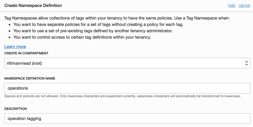
Once created the namespace, we can then create the set of keys within it. In this case, we create two pre-defined keys Environment and Project, please note that we flagged the COST-TRACKING checkbox to be able to use the tags with the Oracle Cloud Account Metering APIs.
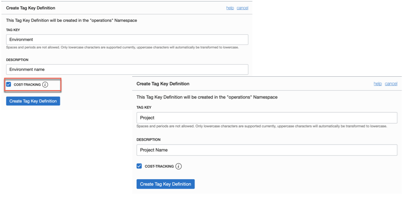
Please be aware that there are limits on the number of namespaces, of tags per resource and of cost-tracking tags which are available under the tagging documentation.
Now it's time to attach the defined tags to our instances, we can do so in the web UI during instance creation or after by selecting "Add Tags". More information under the related documentation.
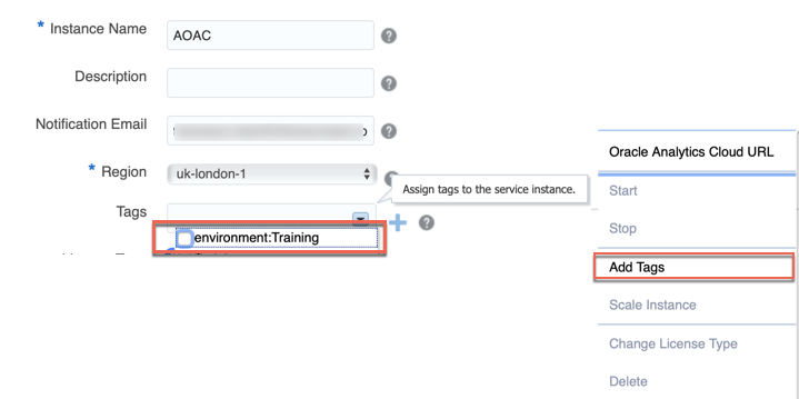
After we added the tags marked for cost-tracking to our instances we may have to wait up to 5 hours to see them in the "My Services" or via the REST APIs.
Querying Tagged Resources
There is an API within the Oracle Cloud Account Metering REST APIs which allows to querying the cost associated with tagged resources. The call is very similar to the one we used above, with the additional tagged prefix and tags=.... parameter. Taking the example above, if we can see the consumption associated with instances tagged as Operations:Project=Training then the call is the following
curl -X GET -u <USERNAME>:<PASSWORD> \
	-H "X-ID-TENANT-NAME:<TENANT_ID>" \
	"https://itra.oraclecloud.com/metering/api/v1/usagecost/<ACCOUNT_ID>/tagged?startTime=<START>&endTime=<END>&timeZone=<TZ>&tags=operations:Project=Training"
And the result is
{
  "accountId": "<ACCOUNT_ID>",
  "items": [
    {
      "subscriptionId": "...",
      "subscriptionType": "PRODUCTION",
      "serviceName": "ADWC",
      "resourceName": "ADWC_PAAS_BYOL_OCPU_HOUR",
      "currency": "GBP",
      "gsiProductId": "B89039",
      "startTimeUtc": "2019-08-01T00:00:00.000",
      "endTimeUtc": "2019-08-10T23:00:00.000",
      "serviceEntitlementId": "...",
      "costs": [
        {
          "computedQuantity": 23.0,
          "computedAmount": 8.06235468,
          "unitPrice": 0.35053716,
          "overagesFlag": "N"
        }
      ]
    }
  ],
  "canonicalLink": "/metering/api/v1/usagecost/<ACCOUNT_ID>/tagged?timeZone=UTC&startTime=2019-08-01T00%3A00%3A00.000Z&endTime=2019-08-10T23%3A59%3A00.000Z&usageType=TOTAL&tags=operations%3AProject%3DTraining"
}
A usage of ADWC for 23 hours for a total of £8.06 which is also visible from the My Services webpage.
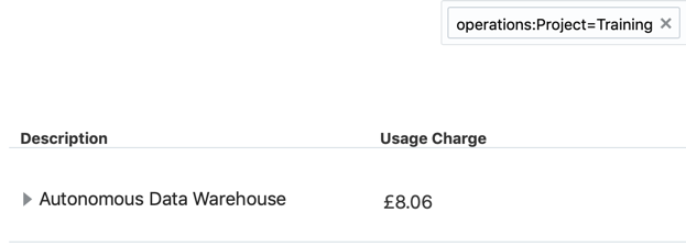
Appending the following jq command to the cURL call also displays the relevant information like serviceName, and cost details as separate columns
jq --raw-output '.items[] | "\(.serviceName)\t\(.subscriptionType)\t\(.resourceName)\t\(.currency)\t\(.costs[].computedAmount)\t\(.costs[].computedQuantity)\t\(.costs[].unitPrice)\t\(.costs[].overagesFlag)"' And the result is
ADWC PRODUCTION ADWC_PAAS_BYOL_OCPU_HOUR GBP 8.06235468 23 0.35053716 NSummary
Oracle Cloud Account Metering REST APIs offer an easy way to expose the Oracle cloud usage and cost externally. Used smartly in conjunction with instance tagging they provide a way to ensure cost and usage tracking down to the single resource or project.
If on the other way, the integration with REST APIs is not what you need, but you're looking into ways of getting notified when you're spending too much, check out the Alerts section of Managing and Monitoring Oracle Cloud.
KSQL in Football: FIFA Women’s World Cup Data Analysis
One of the football (as per European terminology) highlights of the summer is the FIFA Women’s World Cup. France, Brazil, and the USA are the favourites, and this year Italy is present at the event for the first time in 20 years.
From a data perspective, the World Cup represents an interesting source of information. There's a lot of dedicated press coverage, as well as the standard social media excitement following any kind of big event.
The idea in this blog post is to mix information coming from two distinct channels: the RSS feeds of sport-related newspapers and Twitter feeds of the FIFA Women’s World Cup. The goal will be to understand how the sentiment of official news related to the two teams involved in the final compares to that of the tweets.
In order to achieve our targets, we'll use pre-built connectors available in Confluent Hub to source data from RSS and Twitter feeds, KSQL to apply the necessary transformations and analytics, Google’s Natural Language API for sentiment scoring, Google BigQuery for data storage, and Google Data Studio for visual analytics.
Data sources
The beginning of our journey starts with connecting to various data sources. Twitter represents the default source for most event streaming examples, and it's particularly useful in our case because it contains high-volume event streaming data with easily identifiable keywords that can be used to filter for relevant topics.
Ingesting Twitter data
Ingesting Twitter data is very easy with Kafka Connect, a framework for connecting Kafka with external systems. Within the pre-built connectors we can find the Kafka Connect Twitter, all we need to do is install it using the Confluent Hub client.
confluent-hub install jcustenborder/kafka-connect-twitter:latestTo start ingesting the Twitter data, we need to create a configuration file containing the following important bits:
filter.keywords: We need to list all the keywords we are interested in, separated by a comma. Since we want to check tweets from the FIFA Women’s World Cup, we’ll useFIFAWWC, representing both the World Cup Twitter handle and the most common related hashtag.kafka.status.topic: This topic that will be used to store the tweets we selected. twitter_avro: This is because the connector output format is AVRO.twitter.oauth: This represents Twitter credentials. More information can be found on the Twitter’s developer website.
After the changes, our configuration file looks like the following:
filter.keywords=FIFAWWC
kafka.status.topic=twitter_avro
twitter.oauth.accessToken=<TWITTER ACCESS TOKEN>
twitter.oauth.accessTokenSecret=<TWITTER ACCESS TOKEN SECRET>
twitter.oauth.consumerKey=<TWITTER ACCESS CUSTOMER KEY>
twitter.oauth.consumerSecret=<TWITTER CUSTOMER SECRET>
It's time to start it up! We can use the Confluent CLI load command:
confluent load twitter -d $TWITTER_HOME/twitter.properties$TWITTER_HOME is the folder containing the configuration file. We can check the Kafka Connect status by querying the REST APIs with the following:
curl -s "http://localhost:8083/connectors/twitter/status" | jq [.connector.state]
[
  "RUNNING"
]
We can also check if all the settings are correct by consuming the AVRO messages in the twitter_avro topic with a console consumer:
confluent consume twitter_avro --value-format avroAnd the result is, as expected, an event stream of tweets.
RSS feeds as another data source
The second data source that we'll use for our FIFA Women’s World Cup sentiment analytics are RSS feeds from sports-related newspapers. RSS feeds are useful because they share official information about teams and players, like results, episodes, and injuries. RSS feeds should be considered neutral since they should only report facts. For this blog post, we’ll use RSS feeds as a way to measure the average sentiment of the news. As per the Twitter case above, a prebuilt Kafka Connect RSS Source exists, so all we need to do is to install it via the Confluent Hub client:
confluent-hub install kaliy/kafka-connect-rss:latestThen, create a configuration file with the following important parameters:
rss.urls: This is a list of space-separated RSS feed URLs. For our Women’s World Cup example, we’ve chosen the following sources: La Gazzetta dello Sport, Transfermarkt, Eurosport, UEFA, The Guardian, Daily Mail, The Sun Daily, BBCtopic: The Kafka topic to write to, which is rss_avro in our case
The full configuration file looks like the following:
name=RssSourceConnector
tasks.max=1
connector.class=org.kaliy.kafka.connect.rss.RssSourceConnector
rss.urls=https://www.transfermarkt.co.uk/rss/news https://www.eurosport.fr/rss.xml https://www.uefa.com/rssfeed/news/rss.xml https://www.theguardian.com/football/rss https://www.dailymail.co.uk/sport/index.rss https://www.thesundaily.my/rss/sport http://feeds.bbci.co.uk/news/rss.xml https://www.gazzetta.it/rss/home.xml
topic=rss_avro
And again, we can start the ingestion of RSS feeds with the Confluent CLI:
confluent load RssSourceConnector -d $RSS_HOME/RssSourceConnector.propertiesWe can test the status of Kafka Connectors using this simple procedure, and calling it like:
./connect_status.sh
RssSourceConnector  |  RUNNING  |  RUNNING
twitter             |  RUNNING  |  RUNNING
We can see that the both the RssSourceConnector and the twitter Connect are up and running. We can then check the actual data with the console consumer.
confluent consume rss_avro --value-format avroBelow is the output as expected.
Shaping the event streams
After ingesting the Twitter and RSS event streams into topics, it’s time to shape them with KSQL. Shaping the topics accomplishes two purposes:
- It makes the topics queryable from KSQL
- It defines additional structures that can be reused in downstream applications
The Twitter stream lands in Avro format with the fields listed in the related GitHub repo. We can easily declare a TWITTER_STREAM KSQL stream on top of TWITTER_AVRO with:
CREATE STREAM TWITTER_STREAM WITH (
KAFKA_TOPIC='TWITTER_AVRO',
VALUE_FORMAT='AVRO',
TIMESTAMP='CREATEDAT'
);
There is no need to define the single fields in the event stream declaration because they are already in AVRO and thus will be sourced from the Confluent Schema Registry. Schema Registry is the component within Kafka, in charge of storing, versioning and serving the topics Avro Schemas. When a topic is in AVRO format, its schema is stored in the Schema Registry, where downstream applications (like KSQL in this case) can retrieve it and use it to “shape” the messages in the topic.
The important bits of the above KSQL for our definition are:
KAFKA_TOPIC='TWITTER_AVRO': the definition of the source topicVALUE_FORMAT='AVRO': the definition of the source topic formatTIMESTAMP='CREATEDAT': the Tweet's creation date, which is used as the event timestamp
We can now check that the fields’ definition has correctly been retrieved by the Schema Registry with:
DESCRIBE TWITTER_STREAM;Or, we can use the REST API by:
curl -X "POST" "http://localhost:8088/ksql" \
-H "Content-Type: application/vnd.ksql.v1+json; charset=utf-8" \
-d $'{
"ksql": "DESCRIBE TWITTER_STREAM;",
"streamsProperties": {}
}'
The resulting fields section will be:
"fields": [
{
"name": "ROWTIME",
"schema": {
"type": "BIGINT",
"fields": null,
"memberSchema": null
},
{
"name": "ROWKEY",
"schema": {
"type": "STRING",
"fields": null,
"memberSchema": null
},
{
"name": "CREATEDAT",
"schema": {
"type": "BIGINT",
"fields": null,
"memberSchema": null
},
{
"name": "ID",
"schema": {
"type": "BIGINT",
"fields": null,
"memberSchema": null
},
...
}
The same applies to the RSS feed contained in rss_avro with:
create stream RSS_STREAM
WITH(
KAFKA_topic='rss_avro',
TIMESTAMP='DATE',
TIMESTAMP_FORMAT='yyyy-MM-dd''T''HH:mm:ss''Z''',
VALUE_FORMAT='AVRO'
)
The result will be:
ksql> describe RSS_STREAM;
Name                 : RSS_STREAM
Field   | Type
--------------------------------------------------------------
ROWTIME | BIGINT           (system)
ROWKEY  | VARCHAR(STRING)  (system)
FEED    | STRUCT<TITLE VARCHAR(STRING), URL VARCHAR(STRING)>
TITLE   | VARCHAR(STRING)
ID      | VARCHAR(STRING)
LINK    | VARCHAR(STRING)
CONTENT | VARCHAR(STRING)
AUTHOR  | VARCHAR(STRING)
DATE    | VARCHAR(STRING)
--------------------------------------------------------------
We can also use the URL manipulation functions added in KSQL 5.2 to extract useful information from the LINK column with:
CREATE STREAM RSS_STREAM_URL_DECODING AS
SELECT LINK,
URL_EXTRACT_HOST(LINK) HOST,
URL_EXTRACT_PATH(LINK) PATH,
URL_EXTRACT_PROTOCOL(LINK) PROTOCOL,
URL_EXTRACT_QUERY(LINK) QUERY_TEXT
FROM RSS_STREAM;
The result will be:
ksql> SELECT HOST, PATH, PROTOCOL, QUERY_TXT FROM RSS_STREAM_URL_DECODING LIMIT 5;
www.dailymail.co.uk | /sport/football/article-6919585/Paul-Scholes-backs-Manchester-United-spring-surprise-Barcelona.html | https | ns_mchannel=rss&ns_campaign=1490&ito=1490
www.dailymail.co.uk | /sport/formulaone/article-6916337/Chinese-Grand-Prix-F1-race-LIVE-Shanghai-International-Circuit.html | https | ns_mchannel=rss&ns_campaign=1490&ito=1490
www.dailymail.co.uk | /sport/football/article-6919403/West-Brom-make-approach-Preston-manager-Alex-Neil.html | https | ns_mchannel=rss&ns_campaign=1490&ito=1490
www.dailymail.co.uk | /sport/football/article-6919373/Danny-Murphy-Jermaine-Jenas-fascinating-mind-games-thrilling-title-race.html | https | ns_mchannel=rss&ns_campaign=1490&ito=1490
www.dailymail.co.uk | /sport/football/article-6919215/Brazilian-legend-Pele-successfully-undergoes-surgery-remove-kidney-stone-Sao-Paulo-hospital.html | https | ns_mchannel=rss&ns_campaign=1490&ito=1490
Limit Reached
Query terminated
Sentiment analytics and Google’s Natural Language APIs
Text processing is a part of machine learning and is continuously evolving with a huge variety of techniques and related implementations. Sentiment analysis represents a branch of text analytics and aims to identify and quantify affective states contained in a text corpus.
Natural Language APIs provide sentiment scoring as a service using two dimensions:
- Score: Positive (Score > 0) or Negative (Score < 0) Emotion
- Magnitude: Emotional Content Amount
For more information about sentiment score and magnitude interpretation, refer to the documentation.
Using Natural Language APIs presents various benefits:
- Model training: Natural Language is a pre-trained model, ideal in situations where we don't have a set of already-scored corpuses.
- Multi-language: RSS feeds and tweets can be written in multiple languages. Google Natural Language is capable of scoring several languages natively.
- API call: Natural Language can be called via an API, making the integration easy with other tools.
Sentiment scoring in KSQL with user- defined functions (UDFs)
The Natural Language APIs are available via client libraries in various languages, including Python, C#, and Go. For the purposes of this blog post, we'll be looking at the Java implementation since it is currently the language used to implement KSQL user-defined functions (UDFs). For more details on how to build a UD(A)F function, please refer to How to Build a UDF and/or UDAF in KSQL 5.0 by Kai Waehner, which we'll use as base for the GSentiment class definition.
The basic steps to implementing Natural Language API calls in a UDF are the following:
- Add the google.cloud.language JAR dependency in your project. If you are using Maven, you just need to add the following in your
pom.xml
<dependency>: <groupId>com.google.cloud</groupId> <artifactId>google-cloud-language</artifactId> <version>1.25.0</version> </dependency>
- Create a new Java class called GSentiment.
- Import the required classes:
//KSQL UDF Classes import io.confluent.ksql.function.udf.Udf; import io.confluent.ksql.function.udf.UdfDescription; //Google NL Classes import com.google.cloud.language.v1.LanguageServiceClient; import com.google.cloud.language.v1.Sentiment; import com.google.cloud.language.v1.AnalyzeSentimentResponse; import com.google.cloud.language.v1.Document; import com.google.cloud.language.v1.Document.Type;
- Define the
GSentimenclass and add the Java annotations@UdfDescription(name = "gsentiment", description = "Sentiment scoring using Google NL API") public class Gsentiment { ... }. - Within the class, declare
gsentimentas the method accepting aStringtext as input. As of now, UDFs can't return two output values, so we are returning the sentiment score and magnitude as an array of double.@Udf(description = "return sentiment scoring") public List<Double> gsentiment( String text) { ... }. - Within the gsentiment method, invoke the Natural Language API sentiment and cast the result as an array. Since a UDF can return only one parameter currently, we need to pipe the sentiment score and magnitude into an array of two elements.
Double[] arr = new Double[2];
try (LanguageServiceClient languageServiceClient = LanguageServiceClient.create()) {
Document document = Document.newBuilder()
                .setContent(text)
                .setType(Type.PLAIN_TEXT)
                .build();
AnalyzeSentimentResponse response = languageServiceClient.analyzeSentiment(document);
Sentiment sentiment = response.getDocumentSentiment();

arr[0]=(double)sentiment.getMagnitude();
arr[1]=(double)sentiment.getScore();
}
catch (Exception e) {
arr[0]=(double) 0.0;
arr[1]=(double) 0.0;
}
return Arrays.asList(arr);
- As mentioned in How to Build a UDF and/or UDAF in KSQL 5.0, build an uber JAR that includes the KSQL UDF and any dependencies, and copy it to the KSQL extension directory (defined in the
ksql.extension.dirparameter inksql-server.properties). - Add an environment variable
GOOGLE_APPLICATION_CREDENTIALSpointing to the service account key that will be used to authenticate to Google services. - Restart KSQL.
At this point, we should be able to call the GSentiment UDF from KSQL:
ksql> SELECT GSENTIMENT(text) FROM TWITTER_STREAM LIMIT 5;
[0.10000000149011612, -0.10000000149011612]
[0.20000000298023224, 0.20000000298023224]
[0.5                , 0.10000000149011612]
[0.10000000149011612, 0.10000000149011612]
[0.0                , 0.0]
Limit Reached
Query terminated
As expected, the UDF returns an ARRAY of numbers. In order to get the sentiment score and magnitude in separated columns, we simply need to extract the relevant values:
ksql> SELECT GSENTIMENT(TEXT)[0] SCORE, GSENTIMENT(TEXT)[1] MAGNITUDE FROM TWITTER_STREAM LIMIT 5;
0.20000000298023224 | 0.10000000149011612
0.30000001192092896 | 0.10000000149011612
0.800000011920929   | 0.800000011920929
0.0                 | 0.0
0.30000001192092896 | 0.30000001192092896
Limit Reached
Query terminated
However, we should note that Natural Language APIs are priced per API call and, in the above SQL, we are calling the API two times—one for each GSENTIMENT call. Therefore, the above SQL will cost us two API calls per document. To optimise the cost, we can create a new event stream TWITTER_STREAM_WITH_SENTIMENT, which will physicalize in Kafka the array.
CREATE STREAM TWITTER_STREAM_WITH_SENTIMENT AS
SELECT
*,
GSENTIMENT(TEXT) AS SENTIMENT
FROM TWITTER_STREAM;
Next, parse the sentiment SCORE and MAGNITUDE from the TWITTER_STREAM_WITH_SENTIMENT event stream:
CREATE STREAM TWITTER_STREAM_WITH_SENTIMENT_DETAILS as
SELECT *,
SENTIMENT[0] SCORE,
SENTIMENT[1] MAGNITUDE
FROM TWITTER_STREAM_WITH_SENTIMENT;
With this second method, we optimize the cost with a single Natural Language API call per tweet. We can do the same with the RSS feeds by declaring:
CREATE STREAM RSS_STREAM_WITH_SENTIMENT AS
SELECT
*,
GSENTIMENT(CONTENT) SENTIMENT
FROM RSS_STREAM_FLATTENED;
CREATE STREAM RSS_STREAM_WITH_SENTIMENT_DETAILS as
SELECT *,
SENTIMENT[0] SCORE,
SENTIMENT[1] MAGNITUDE
FROM RSS_STREAM_WITH_SENTIMENT;
Sink to Google BigQuery
The following part of this blog post focuses on pushing the dataset into Google BigQuery and visual analysis in Google Data Studio.
Pushing the data into BigQuery is very easy—just install the BigQuery Sink Connector with:
confluent-hub install wepay/kafka-connect-bigquery:latestNext, configure it while applying the following parameters (amongst others):
topics: defines the topic to read (in our caseRSS_STREAM_WITH_SENTIMENT_DETAILSandTWITTER_STREAM_WITH_SENTIMENT_DETAILS)project: the name of the Google project that we’ll use for billingdatasets=.*=wwc: defines the BigQuery dataset namekeyfile=$GOOGLE_CRED/myGoogleCredentials.json: points to the JSON file containing Google's credentials (which in our case is the same file used in the Google Natural Language scoring)
Before starting the connector, we need to ensure the BigQuery dataset named wwc (as per configuration file) exists, otherwise, the connector will fail. To do so, we can log into BigQuery, select the same project defined in the configuration file, and click on CREATE DATASET. Then, we’ll need to fill in all the details (more information about the dataset creation in the Google documentation).
After creating the dataset, it’s time to start the connector with the Confluent CLI:
confluent load bigquery-connector -d $RSS_HOME/connectorBQ.propertiesIf the Kafka sink works, we should see one table per topic defined in the configuration file, which are RSS_STREAM_WITH_SENTIMENT_DETAILS and TWITTER_STREAM_WITH_SENTIMENT_DETAILS in our case.
Of course, we can query the data from BigQuery itself.
Visual Analysis in Google Data Studio
To start analysing the data in Google Data Studio, simply connect to the related console and select “Blank Report.”
We’ll be asked which data source to use for the project. Thus, we need to set up a connection to the wwc dataset by clicking on CREATE NEW DATASOURCE and selecting BigQuery as the connection. Then, select the project, dataset, and table ( TWITTER_STREAM_WITH_SENTIMENT_DETAILS).
We can then review the list of columns, types, and aggregations, adding the data source to the report.
Finally, we can start creating visualisations like tiles to show record counts, line charts for the sentiment trend, and bar charts defining the most used languages.
A more advanced visualisation like a scatterplot shows the most common hashtags and the associated average sentiment value.
Below is a map visualising the average sentiment by country.
Analysing and comparing sentiment scores
Now that we have the two streams of data coming from Twitter and RSS feeds, we can do the analysis in KSQL and, in parallel, visually in Google Data Studio. We can, for example, examine the average sentiment over a timeframe and check how one source sentiment score compares to the other.
On the 27th of June, the quarterfinal match between Norway and England was played, with the result being that England beat Norway 3–0. Let’s check if we can somehow find significant similarities in the sentiment scoring of our dataset.
Starting with the Twitter feed, we can check all the tweets including ENGLAND and NORWAY by filtering the related hashtag #NORENG. To obtain the team related overall score, I’m then assigning to each team all the tweets containing the country full name and aggregating the SENTIMENTSCORE with the following SQL:
CREATE STREAM TWITTER_NORWAY_ENGLAND AS
SELECT
CASE
WHEN UCASE(TEXT) LIKE '%NORWAY%' THEN SENTIMENTSCORE
END AS NORWAY_SENTIMENTSCORE,
CASE
WHEN UCASE(TEXT) LIKE '%ENGLAND%' THEN SENTIMENTSCORE
END AS ENGLAND_SENTIMENTSCORE
FROM TWITTER_STREAM_WITH_SENTIMENT_DETAILS
WHERE TEXT LIKE '%#NORENG%';
We can check the overall sentiment score associated with the two teams using:
SELECT
SUM(NORWAY_SENTIMENTSCORE)/COUNT(NORWAY_SENTIMENTSCORE) AS NORWAY_AVG_SCORE,
SUM(ENGLAND_SENTIMENTSCORE)/COUNT(ENGLAND_SENTIMENTSCORE) AS ENGLAND_AVG_SCORE
FROM TWITTER_NORWAY_ENGLAND
GROUP BY 1;
The GROUP BY 1 is necessary since KSQL currently requires a GROUP BY clause when using aggregation functions like SUM. Since we don’t aggregate for any columns other than the window time, we can use the number 1 as fix aggregator for the total. The result of the above query is in line with the final score, with the winner (England) having an average sentiment score of 0.212, and the loser (Norway) having a score of 0.0979.
We can also look at the behaviour per hour with the TUMBLING KSQL windowing function:
SELECT
TIMESTAMPTOSTRING(WINDOWSTART(), 'EEE dd MMM HH') AS START_WINDOW,
SUM(NORWAY_SENTIMENTSCORE)/COUNT(NORWAY_SENTIMENTSCORE) AS NORWAY_AVG_SCORE,
SUM(ENGLAND_SENTIMENTSCORE)/COUNT(ENGLAND_SENTIMENTSCORE) AS ENGLAND_AVG_SCORE
FROM TWITTER_NORWAY_ENGLAND
WINDOW TUMBLING(SIZE 1 HOURS)
GROUP BY 1;
The query yields the following result:
Thu 27 Jun 16 | 0.18409091 | 0.16075758
Thu 27 Jun 17 | 0.14481481 | 0.13887096
Thu 27 Jun 18 | 0.14714406 | 0.12107647
Thu 27 Jun 19 | 0.07926398 | 0.34757579
Thu 27 Jun 20 | 0.10077705 | 0.13762544
Thu 27 Jun 21 | 0.08387538 | 0.17832865
We can clearly see that towards match time (19:00 BST), the ENGLAND average score has a spike, in coincidence with England’s first goal in the third minute. We can see the same on the Line Chart in Google Data Studio.
We can do a similar exercise on top of the RSS feeds stream, but first, we need to somehow filter it to get only FIFA Women’s World Cup 2019 data, since the predefined connector is ingesting all the news from the RSS sources without a topic filter. To do so, we create a new stream filtering only contents containing WOMEN and CUP:
CREATE STREAM RSS_STREAM_WITH_SENTIMENT_DETAILS_WWC as
SELECT *
FROM RSS_STREAM_WITH_SENTIMENT_DETAILS
WHERE UCASE(CONTENT) LIKE '%WOMEN%'
AND UCASE(CONTENT) LIKE '%CUP%';
We can now analyse the overall RSS sentiment with:
SELECT SUM(SENTIMENTSCORE)/COUNT(SENTIMENTSCORE)
FROM RSS_STREAM_WITH_SENTIMENT_DETAILS_WWC
GROUP BY 1;
As before, the SUM(SENTIMENTSCORE)/COUNT(SENTIMENTSCORE) is calculating the average. We can then calculate the sentiment average for the selected team. Taking the same example of ENGLAND and NORWAY used previously, we just declare a stream filtering the sentiment for the two nations. For example:
CREATE STREAM RSS_NORWAY_ENGLAND AS
SELECT
CASE WHEN UCASE(CONTENT) LIKE '%NORWAY%' THEN SENTIMENTSCORE END NORWAY_SENTIMENTSCORE,
CASE WHEN UCASE(CONTENT) LIKE '%ENGLAND%' THEN SENTIMENTSCORE END ENGLAND_SENTIMENTSCORE
FROM RSS_STREAM_WITH_SENTIMENT_DETAILS_WWC;
Then, we can analyse the separate scoring with:
SELECT
SUM(NORWAY_SENTIMENTSCORE)/COUNT(NORWAY_SENTIMENTSCORE) NORWAY_AVG_SENTIMENT,
SUM(ENGLAND_SENTIMENTSCORE)/COUNT(ENGLAND_SENTIMENTSCORE) ENGLAND_AVG_SENTIMENT
FROM RSS_NORWAY_ENGLAND
WHERE ROWTIME > STRINGTODATE('2019-06-27', 'yyyy-MM-dd')
GROUP BY 1;
The result is an average sentiment of 0.0575 for Norway and 0.111 for England, again in line with the match result where England won 3–0.
We can also understand the variation of the sentiment over time by using KSQL windowing functions like TUMBLING:
SELECT
TIMESTAMPTOSTRING(WINDOWSTART(), 'EEE dd MMM HH') START_WINDOW,
SUM(NORWAY_SENTIMENTSCORE)/COUNT(NORWAY_SENTIMENTSCORE) NORWAY_AVG_SENTIMENT,
SUM(ENGLAND_SENTIMENTSCORE)/COUNT(ENGLAND_SENTIMENTSCORE) ENGLAND_AVG_SENTIMENT
FROM RSS_NORWAY_ENGLAND WINDOW TUMBLING(SIZE 1 HOURS)
WHERE ROWTIME >= STRINGTODATE('2019-06-27', 'yyyy-MM-dd')
GROUP BY 1;
This yields the following results:
Thu 27 Jun 17 | 0.12876364 | 0.12876364
Thu 27 Jun 18 | 0.24957054 | 0.24957054
Thu 27 Jun 19 | 0.15606978 | 0.15606978
Thu 27 Jun 20 | 0.09970317 | 0.09970317
Thu 27 Jun 21 | 0.00809077 | 0.00809077
Thu 27 Jun 23 | 0.41298701 | 0.12389610
As expected from this source, most of the scoring of the two countries are the same since the number of articles is limited and almost all articles mention both ENGLAND and NORWAY.
Strangely, as we can see in the graph above, the NORWAY sentiment score on the 27th of June at 11:00 pm GMT (so after the match ended) is much higher than the ENGLAND one.
We can look at the data closely with:
SELECT ROWKEY, NORWAY_SENTIMENTSCORE, ENGLAND_SENTIMENTSCORE
from NORWAY_ENGLAND where TIMESTAMPTOSTRING(ROWTIME,'dd/MM HH') = '27/06 23';
https://www.theguardian.com/...      | 0.375974032  | 0.375974032
https://www.bbc.co.uk/.../48794550   | null         | -0.45428572
https://www.bbc.co.uk/.../48795487   | 0.449999988  | 0.449999988
We can see that NORWAY is being associated with two articles: one from The Guardian with a positive 0.375 score and one from BBC with a positive 0.449 score. ENGLAND, on the other hand, is associated with another BBC article, having a negative -0.454 score.
We can also compare the hourly Twitter and RSS sentiment scores by creating two tables:
CREATE TABLE TWITTER_NORWAY_ENGLAND_TABLE AS
SELECT
TIMESTAMPTOSTRING(WINDOWSTART(), 'dd HH') START_WINDOW,
SUM(NORWAY_SENTIMENTSCORE)/COUNT(NORWAY_SENTIMENTSCORE) NORWAY_AVG_SCORE,
SUM(ENGLAND_SENTIMENTSCORE)/COUNT(ENGLAND_SENTIMENTSCORE) ENGLAND_AVG_SCORE
FROM TWITTER_NORWAY_ENGLAND
WINDOW TUMBLING(SIZE 1 HOURS)
GROUP BY 1;
CREATE TABLE RSS_NORWAY_ENGLAND_TABLE AS
SELECT
TIMESTAMPTOSTRING(WINDOWSTART(), 'dd HH') START_WINDOW,
SUM(NORWAY_SENTIMENTSCORE)/COUNT(NORWAY_SENTIMENTSCORE) NORWAY_AVG_SCORE,
SUM(ENGLAND_SENTIMENTSCORE)/COUNT(ENGLAND_SENTIMENTSCORE) ENGLAND_AVG_SCORE
FROM NORWAY_ENGLAND WINDOW TUMBLING(SIZE 1 HOURS)
WHERE ROWTIME >= STRINGTODATE('2019-06-27', 'yyyy-MM-dd')
GROUP BY 1;
The key of both the tables is the window start date, as we can see from:
ksql> select rowkey from RSS_NORWAY_ENGLAND_TABLE limit 1;
1 : Window{start=1561557600000 end=-}
We can then join the results together with the following statement:
SELECT A.START_WINDOW,
A.NORWAY_AVG_SENTIMENT TWITTER_NORWAY_SCORE,
A.ENGLAND_AVG_SENTIMENT TWITTER_ENGLAND_SCORE,
B.NORWAY_AVG_SENTIMENT RSS_NORWAY_SCORE,
B.ENGLAND_AVG_SENTIMENT RSS_ENGLAND_SCORE
FROM
TWITTER_NORWAY_ENGLAND_TABLE A JOIN
RSS_NORWAY_ENGLAND_TABLE B
ON A.ROWKEY = B.ROWKEY;
This yields the following result:
Thu 27 Jun 17 | 0.14481481 | 0.13887096 | 0.12876364 | 0.12876364
Thu 27 Jun 18 | 0.14714406 | 0.12107647 | 0.24957054 | 0.24957054
Thu 27 Jun 19 | 0.07926398 | 0.34757579 | 0.15606978 | 0.15606978
Thu 27 Jun 20 | 0.10077705 | 0.13762544 | 0.09970317 | 0.09970317
Thu 27 Jun 21 | 0.08387538 | 0.17832865 | 0.00809077 | 0.00809077
And the end result similarly in a Data Studio Line Chart
Interested in more?
If you’re interested in what KSQL can do, you can download the Confluent Platform to get started with the event streaming SQL engine for Apache Kafka. To help you get started, Rittman Mead provides a 30 day Kafka quick start package
This article was originally posted on the Confluent blog.
Kafka and Football: KSQL, Google Natural Language APIs, BigQuery and DataStudio
If you missed it, yesterday I wrote a guest blog post for Confluent! The blog post mixes two of my favorite topics: Apache Kafka and Football! The post starts by defining the data ingestion from Twitter and sport news RSS feeds via Kafka Connect, continues with the definition of a KSQL UDF Function using Google Natural Language APIs for Sentiment Analysis. Then it's time to define the data sink to Google Big Query and the data visualization with Google Data Studio.
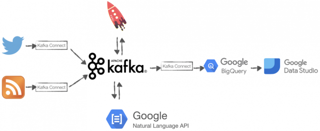
The last bit of the post is dedicated to data analysis with both KSQL and DataStudio on top of the quarterfinal match won by England against Norway. If you are interested in the full article, check it out here!
Oracle Analytics Summit 2019
Last week I attended the Oracle Analytics Summit at Skywalker Ranch. The event was live-streamed on Facebook and widely Tweeted, so a fair number of people may be up to speed with the announcements, I’ll summarise what I thought the key points were.
The purpose of the event, I think, was to relaunch/re-energise Oracle’s analytics products and services, make some specific announcements, and to try and better engage customers and analysts.
I think a lot of this stems from T. K. Anand taking over last summer and the changes in the team and direction he is looking to make. He was the first speaker at talked of openness and simplicity.
New Product Line
First, he announced a rationalisation of the product line with three offerings:
- OAC (Oracle Analytics Cloud) - this is OAC on the second generation OCI (Oracle Cloud Infrastructure), with a simpler pricing model, details below.
- OAS (Oracle Analytics Server) - this is a feature parity version of OAC available on premise.
- OAA (Oracle Analytics Applications) - this is a new ‘BI Apps’ product for Oracle’s SaaS offerings such as ERP Cloud and HCM Cloud, more details below.
New Pricing
Second, he announced new pricing for OAC:
- $20/month for Professional Edition
- $2,000/month per OCPU for Enterprise Edition
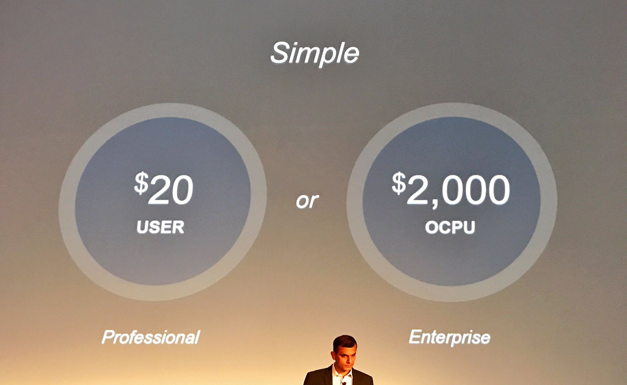
Image from Doug Henschen
This also streamlined the different versions of OAC. Professional is essentially DV (Data Visualisation), and Enterprise is OBIEE and DV. I am not sure what this means for the existing Data Lake edition, however, I believe Essbase is being moved to a separate PaaS service.
I believe this also means that in the future if you are an on-premise OAS customer with the Enterprise Edition, then DV will be included in the price.
At the time of writing this, I’m not sure of the minimum number of users for the Professional Edition, however, given the price point, it looks like Oracle are targeting Power BI, Tableau etc., so I would expect a low number.
The Future of BI Apps
BI Apps has risen from the flames, and I believe there are now a couple of options:
- The existing ODI ‘version’ of BI Apps is being updated to support ODI 12c, OBIEE 12c/OAC and ADW. This means whether you have your application reporting on-premise or in the cloud, there is an upgrade path for the traditional BI Apps components, plus, due to the support of ADW, you will be able to migrate an existing on-premise system to Oracle’s cloud. Independent of anything that happens to DIPC, ODI will be supported on Oracle’s IaaS.
- There is a new cloud-only version of packaged applications, see OAA above. These provide a managed data pipeline between the SaaS application and an instance of ADW. Information is surfaced through what looks like DV, with some extended capabilities, allowing KPIs to be defined and these KPIs to arranged as a series of Tiles on a dashboard, not unlike the look of the Day by Day app.
Customer Commitment
One clear objective is more interaction and integration with customers, and to this end Oracle is increasing the number of people in support, there is more online content available, such as their Udemy channel and they are also creating something called the Idea Lab for the analytics community, where users can make suggestions and interact with the Product Managers.
Summary
I felt throughout the event that Oracle are aware of their shortcomings in the past and are committed to listening to customers, giving them a better experience and putting them more at the centre of their world.
The product line and pricing changes act as proof that they are committed to acting on this; it’s not just lip service. Through the pricing of the Professional Edition, I think you can also see Oracle going for the departmental or shadow IT world of data exploration and visualisation.
One customer commented at the end of the event that no one tried to sell him anything, that, if anything, is a good indicator for change.
Rittman Mead at Kscope 2019
June is time for one of my favourite conferences: Kscope! This year the location is Seattle and the Agenda is impressive. The event starts on Sunday with the Symposiums driven by Oracle Product Managers and divided by stream of interest.
The main conference is Monday-Wednesday with the Thursday dedicated to Deep Dive sessions. On Tuesday morning the Analytics track attention will be shifted to Skywalker Ranch for live-stream of the Oracle Analytics Summit!
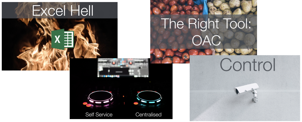
I'll be representing Rittman Mead with two talks: One about "Become an Equilibrista: Find the Right Balance in the Analytics Tech Ecosystem" (Jun 24, 2019 03:45 PM - 04:45 PM, Room 3B, Level 3) discussing how to make self-service and centralized Analytics coexist successfully thus avoiding the "Excel Hell".

The second session is about two topics I love: Machine Learning and Wine! The "Is It Corked? Wine Machine Learning Predictions with OAC" (Jun 25, 2019 03:45 PM - 04:45 PM, Room 3B, Level 3) will show the details on how Oracle Analytics Cloud democratizes data science using a Wine Dataset as example. During the session we'll explore how OAC provides an easy and visual interface to Machine Learning and how a predictive model can be built, tested and evaluated within the same platform.

If you'll be at Kscope 2019 and you see me around, don't hesitate to stop me! I’d be pleased to speak with you about Wine, Food, Coffee, and Analytics of course!


