Author Archives: Rittmanmead
A Performance Analytics Application Case Study: Challenges and Successes
The Performance Analytics application is a collection of open source technologies that aids users in: identifying performance bottlenecks, identifying causes for slow report execution, discovering areas for performance optimization, and gathering meaningful insights into the health of an OBIEE environment.
This post focuses on lessons learned after a successful Performance Analytics application installation, where within one day of being operational it enabled us to identify and isolate a long-standing memory issue. Here's how.

Overview
Rittman Mead recently undertook an engagement with the remit to:
- Carry out a health check on the current state of an OBIEE platform, architecture, and development process
- Install the Rittman Mead Performance Analytics application, enabling rapid and accurate diagnostics of OBIEE issues
The client was on OBIEE 11g, having previously upgraded from 10g. OBIEE Production environment was a three-node cluster running the latest version of the 11g release. It served around 150 users daily, of a registered user base of around 1000.
The client had a long-standing issue with memory alerts on the master node of OBIEE cluster, but no evident architectural, hardware capacity, or software configuration issues were found after completing the health check.
Challenges and successes
Gather all relevant data
Performance Analytics gathers data from a variety of sources in order to provide a full stack view of the OBIEE environment.
Active Session History (ASH) - The Active Session History data is read from the v$ACTIVE_SESSION_HISTORY system database view. Access to this data allows Performance Analytics users to have an understanding of the performance and state of the database at a given point it time as it provides information such as the SQL operation being performed, which application is executing the query, whether the query is actively being performed or is waiting for service, what state of execution the query is in, and many other useful statistics.
Operating System Metrics - Unix-based Operating Systems contain several commands used to gather information about the performance or status of the server such as vmstat, iostat, netstat, top and df. Performance Analytics utilizes the output of these commands to display the current status of the OS at a given point in time.
Usage Tracking - The Oracle BI Server supports the collection of usage tracking data. When usage tracking is enabled, the Oracle BI Server collects usage tracking data for each query, and it writes statistics to a usage tracking log file or inserts them directly into a database table. Access to this data allows Performance Analytics users to have an understanding of the performance of the BI Server and specific reports in the OBIEE environment at any given point in time.
OBIEE metrics - OBIEE has the capability to expose internal performance data through the Dynamic Monitoring Service (DMS). The data exposed contains information such as Connection Pool statistics, JVM statistics, the number of active threads, and much more. Access to this data allows Performance Analytics to record the current status of many of the OBIEE components and intricacies found within the tool.
Performance Analytics was deployed using Docker in a couple of days, requiring absolutely no software installation on any machine other than the monitoring server. All configuration settings are held in one file, and it was sufficient to add connection details of each server to it in order to gather all aforementioned data.
Accurately diagnose issues
By combining operating system metrics (CPU, memory, etc.) with internal OBIEE metrics and those from the database, Performance Analytics gives a "single pane of glass" view on the behaviour of the whole stack. This enables correlations in behaviour to be easily identified, and issues drilled into using the analysis capabilities of the tool.
Within a day of being installed, Performance Analytics enabled the client to accurately diagnose a long-standing issue with memory alerts on OBIEE master node. The cause was traced to the export to Excel of a large dataset by a single user.
Workload Planning
Performance Analytics allows to capture system status and workload over time, so you can see how the system is responding to peak loads in real-time.
With Performance Analytics the client is now able to estimate maximum workload the current architecture can support before starting to see issues and whether it is going to cope with the next years workload.
Conclusion
Performance Analytics just paid for itself.
Performance Analytics collects all relevant data and makes it accessible from one central location, allowing users to investigate performance inquiries promptly and simply. Instead of forcing users to dig through database records or a linux server manually, they can access all of the same data through a set of dashboards engineered to facilitate discovery from the collected data.
If you’d like to find out more about the Performance Analytics service offered by Rittman Mead, please get in touch.
Property Graph in Oracle 12.2
The latest release of Oracle (12.2) includes support for Property Graph, previously available only as part of the Big Data Spatial and Graph tool. Unlike the latter, in which data is held in a NoSQL store (Oracle NoSQL, or Apache HBase), it is now possible to use the Oracle Database itself for holding graph definitions and analysing them.
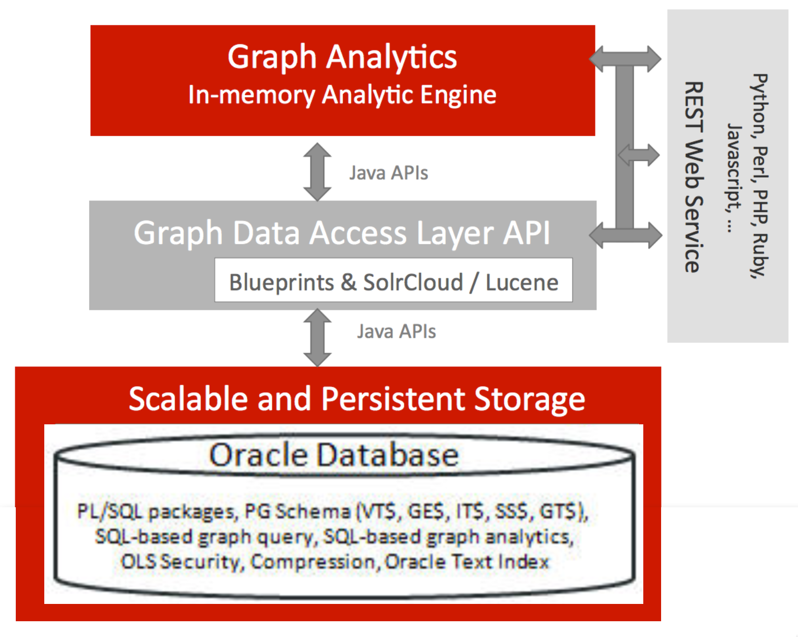
Here we'll see this in action, using the same dataset as I've previously used - the "Panama Papers".
My starting point is the Oracle Developer Day VM, which at under 8GB is a tenth of the size of the beast that is the BigDataLite VM. BDL is great for exploring the vast Big Data ecosystem, both within and external to the Oracle world. However the Developer Day VM serves our needs perfectly here, having been recently updated for the 12.2 release of Oracle. You can also use DB 12.2 in Oracle Cloud, as well as the Docker image.
Prepare Database for Property Graph
The steps below are based on Zhe Wu's blog "Graph Database Says Hello from the Cloud (Part III)", modified slightly for the differing SIDs etc on Developer Day VM.
First, set the Oracle environment by running from a bash prompt
. oraenv
When prompted for SID enter orcl12c:
[oracle@vbgeneric ~]$ . oraenv
ORACLE_SID = [oracle] ? orcl12c
ORACLE_BASE environment variable is not being set since this
information is not available for the current user ID oracle.
You can set ORACLE_BASE manually if it is required.
Resetting ORACLE_BASE to its previous value or ORACLE_HOME
The Oracle base has been set to /u01/app/oracle/product/12.2/db_1
[oracle@vbgeneric ~]$
Now launch SQL*Plus:
sqlplus sys/oracle@localhost:1521/orcl12c as sysdba
and from the SQL*Plus prompt create a tablespace in which the Property Graph data will be stored:
alter session set container=orcl;

create bigfile tablespace pgts
datafile '?/dbs/pgts.dat' size 512M reuse autoextend on next 512M maxsize 10G
EXTENT MANAGEMENT LOCAL
segment space management auto;
Now you need to do a bit of work to update the database to hold larger string sizes, following the following steps.
In SQL*Plus:
ALTER SESSION SET CONTAINER=CDB$ROOT;
ALTER SYSTEM SET max_string_size=extended SCOPE=SPFILE;
shutdown immediate;
startup upgrade;
ALTER PLUGGABLE DATABASE ALL OPEN UPGRADE;
EXIT;
Then from the bash shell:
cd $ORACLE_HOME/rdbms/admin
mkdir /u01/utl32k_cdb_pdbs_output
mkdir /u01/utlrp_cdb_pdbs_output
$ORACLE_HOME/perl/bin/perl $ORACLE_HOME/rdbms/admin/catcon.pl -u SYS -d $ORACLE_HOME/rdbms/admin -l '/u01/utl32k_cdb_pdbs_output' -b utl32k_cdb_pdbs_output utl32k.sql
When prompted, enter SYS password (oracle)
After a short time you should get output:
catcon.pl: completed successfully
Now back into SQL*Plus:
sqlplus sys/oracle@localhost:1521/orcl12c as sysdba
and restart the database instances:
shutdown immediate;
startup;
ALTER PLUGGABLE DATABASE ALL OPEN READ WRITE;
exit
Run a second script from the bash shell:
$ORACLE_HOME/perl/bin/perl $ORACLE_HOME/rdbms/admin/catcon.pl -u SYS -d $ORACLE_HOME/rdbms/admin -l '/u01/utlrp_cdb_pdbs_output' -b utlrp_cdb_pdbs_output utlrp.sql
Again, enter SYS password (oracle) when prompted. This step then takes a while (c.15 minutes) to run, so be patient. Eventually it should finish and you'll see:
catcon.pl: completed successfully
Now to validate that the change has worked. Fire up SQL*Plus:
sqlplus sys/oracle@localhost:1521/orcl12c as sysdba
And check the value for max_string, which should be EXTENDED:
alter session set container=orcl;
SQL> show parameters max_string;

NAME                                 TYPE        VALUE
------------------------------------ ----------- ------------------------------
max_string_size                      string      EXTENDED
Load Property Graph data from Oracle Flat File format
Now we can get going with our Property Graph. We're going to use Gremlin, a groovy-based interpretter, for interacting with PG. As of Oracle 12.2, it ships with the product itself. Launch it from bash:
cd $ORACLE_HOME/md/property_graph/dal/groovy
sh gremlin-opg-rdbms.sh

--------------------------------
Mar 08, 2017 8:52:22 AM java.util.prefs.FileSystemPreferences$1 run
INFO: Created user preferences directory.
opg-oracledb>
First off, let's create the Property Graph object in Oracle itself. Under the covers, this will set up the necessary database objects that will store the data.
cfg = GraphConfigBuilder.\
        forPropertyGraphRdbms().\
        setJdbcUrl("jdbc:oracle:thin:@127.0.0.1:1521/ORCL").\
        setUsername("scott").\
        setPassword("oracle").\
        setName("panama").\
        setMaxNumConnections(8).\
        build();
opg = OraclePropertyGraph.getInstance(cfg);
You can also do this with the PL/SQL command exec opg_apis.create_pg('panama', 4, 8, 'PGTS');. Either way, the effect is the same; a set of tables created in the owner's schema:
SQL> select table_name from user_tables;
TABLE_NAME
------------------------------------------
PANAMAGE$
PANAMAGT$
PANAMAVT$
PANAMAIT$
PANAMASS$
Now let's load the data. I'm using the Oracle Flat File format here, having converted it from the original CSV format using R. For more details of why and how, see my article here.
From the Gremlin prompt, run:
// opg.clearRepository();     // start from scratch
opgdl=OraclePropertyGraphDataLoader.getInstance();
efile="/home/oracle/panama_edges.ope"
vfile="/home/oracle/panama_nodes.opv"
opgdl.loadData(opg, vfile, efile, 1, 10000, true, null);
This will take a few minutes. Once it's completed you'll get null response, but can verify the data has successfully loaded using the opg.Count* functions:
opg-oracledb> opgdl.loadData(opg, vfile, efile, 1, 10000, true, null);
==>null
opg-oracledb> opg.countEdges()
==>1265690
opg-oracledb> opg.countVertices()
==>838295
We can inspect the data in Oracle itself too. Here I'm using SQLcl, which is available by default on the Developer Day VM. Using the ...VT$ table we can query the number of distinct properties the nodes (verticies) in the graph:
SQL> select distinct k from panamaVT$;
K
----------------------------
Entity incorporation.date
Entity company.type
Entity note
ID
Officer icij.id
Countries
Type
Entity status
Country
Source ID
Country Codes
Entity struck.off.date
Entity address
Name
Entity jurisdiction
Entity jurisdiction.description
Entity dorm.date

17 rows selected.
Inspect the edges:
[oracle@vbgeneric ~]$ sql scott/oracle@localhost:1521/orcl

SQL> select p.* from PANAMAGE$ p where rownum<5;

       EID       SVID       DVID EL               K       T V      VN VT     SL VTS  VTE  FE
---------- ---------- ---------- ---------------- ---- ---- ---- ---- ---- ---- ---- ---- ----
         6          6     205862 officer_of
        11         11     228601 officer_of
        30         36     216748 officer_of
        34         39     216487 officer_of

SQL>
You can also natively execute some of the Property Graph algorithms from PL/SQL itself. Here is how to run the PageRank algorithm, which can be used to identify the most significant nodes in a graph, assigning them each a score (the "page rank" value):
set serveroutput on
DECLARE
    wt_pr  varchar2(2000); -- name of the table to hold PR value of the current iteration
    wt_npr varchar2(2000); -- name of the table to hold PR value for the next iteration
    wt3    varchar2(2000);
    wt4    varchar2(2000);
    wt5    varchar2(2000);
    n_vertices number;
BEGIN
    wt_pr := 'panamaPR';
    opg_apis.pr_prep('panamaGE$', wt_pr, wt_npr, wt3, wt4, null);
    dbms_output.put_line('Working table names  ' || wt_pr
       || ', wt_npr ' || wt_npr || ', wt3 ' || wt3 || ', wt4 '|| wt4);
    opg_apis.pr('panamaGE$', 0.85, 10, 0.01, 4, wt_pr, wt_npr, wt3, wt4, 'SYSAUX', null, n_vertices)
;
END;
/
When run this creates a new table with the PageRank score for each vertex in the graph, which can then be queried as any other table:
SQL> select * from panamaPR
  2  order by PR desc
  3* fetch first 5 rows only;
      NODE         PR          C
---------- ---------- ----------
    236724 8851.73652          0
    288469 904.227685          0
    264051 667.422717          0
    285729 562.561604          0
    237076 499.739316          0
On its own, this is not so much use; but joined to the vertices table, we can now find out, within our graph, the top ranked vertices:
SQL> select pr.pr, v.k,v.V from panamaPR pr inner join PANAMAVT$ V on pr.NODE = v.vid where v.K = 'Name' order by PR desc fetch first 5 rows only;
        PR K          V
---------- ---------- ---------------
8851.73652 Name       Portcullis TrustNet Chambers P.O. Box 3444 Road Town- Tortola British Virgin Isl
904.227685 Name       Unitrust Corporate Services Ltd. John Humphries House- Room 304 4-10 Stockwell Stre
667.422717 Name       Company Kit Limited Unit A- 6/F Shun On Comm Bldg. 112-114 Des Voeux Road C.- Hong
562.561604 Name       Sealight Incorporations Limited Room 1201- Connaught Commercial Building 185 Wanc
499.739316 Name       David Chong & Co. Office B1- 7/F. Loyong Court 212-220 Lockhart Road Wanchai Hong K

SQL>
Since our vertices in this graph have properties, including "Type", we can also analyse it by that - the following shows the top ranked vertices that are Officers:
SQL> select V.vid, pr.pr from panamaPR pr inner join PANAMAVT$ V on pr.NODE = v.vid where v.K = 'Type' and v.V = 'Officer' order by PR desc fetch first 5 rows only;
       VID         PR
---------- ----------
  12171184 1.99938104
  12030645 1.56722346
  12169701 1.55754873
  12143648 1.46977361
  12220783 1.39846834
which we can then put in a subquery to show the details for these nodes:
with OfficerPR as
        (select V.vid, pr.pr
          from panamaPR pr
               inner join PANAMAVT$ V
               on pr.NODE = v.vid
         where v.K = 'Type' and v.V = 'Officer'
      order by PR desc
      fetch first 5 rows only)
select pr2.pr,v2.k,v2.v
from OfficerPR pr2
     inner join panamaVT$ v2
     on pr2.vid = v2.vid
where v2.k in ('Name','Countries');
        PR K          V
---------- ---------- -----------------------
1.99938104 Countries  Guernsey
1.99938104 Name       Cannon Asset Management Limited re G006
1.56722346 Countries  Gibraltar
1.56722346 Name       NORTH ATLANTIC TRUST COMPANY LTD. AS TRUSTEE THE DAWN TRUST
1.55754873 Countries  Guernsey
1.55754873 Name       Cannon Asset Management Limited re J006
1.46977361 Countries  Portugal
1.46977361 Name       B-49-MARQUIS-CONSULTADORIA E SERVICOS (SOCIEDADE UNIPESSOAL) LDA
1.39846834 Countries  Cyprus
1.39846834 Name       SCIVIAS TRUST  MANAGEMENT LTD

10 rows selected.
But here we get into the limitations of SQL - already this is starting to look like a bit of a complex query to maintain. This is where PGQL comes in, as it enables to express the above request much more eloquently. The key thing with PGQL is that it understands the concept of a 'node', which removes the need for the convoluted sub-select that I had to do above to first identify the top-ranked nodes that had a given property (Type = Officer), and then for those identified nodes show information about them (Name and Countries). The above SQL could be expressed in PGQL simply as:
SELECT n.pr, n.name, n.countries
WHERE (n WITH Type =~ 'Officer')
ORDER BY n.pr limit 5
At the moment Property Graph in the Oracle DB doesn't support PGQL - but I'd expect to see it in the future.
Jupyter Notebooks
As well as working with the Property Graph in SQL and Gremlin, we can use the Python API. This is shipped with Oracle 12.2. I'd strongly recommend using it through a Notebook, and this provides an excellent environment in which to prototype code and explore the results. Here I'll use Jupyter, but Apache Zeppelin is also very good.
First let's install Anaconda Python, which includes Jupyter Notebooks:
wget https://repo.continuum.io/archive/Anaconda2-4.3.0-Linux-x86_64.sh
bash Anaconda2-4.3.0-Linux-x86_64.sh
In the install options I use the default path (/home/oracle) as the location, and keep the default (no)
Launch Jupyter, telling it to listen on any NIC (not just localhost). If you installed anaconda in a different path from the default you'll need to amend the /home/oracle/ bit of the path.
/home/oracle/anaconda2/bin/jupyter notebook --ip 0.0.0.0
If you ran the above command from the terminal window within the VM, you'll get Firefox pop up with the following:
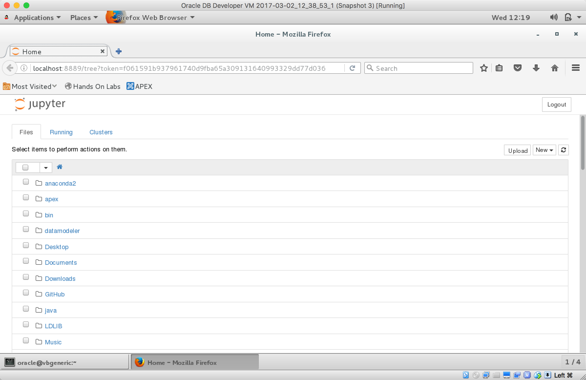
If you're using the VM headless you'll now want to fire up your own web browser and go to http://<ip>:8888 use the token given in the startup log of Jupyter to login.
Either way, you should now have a functioning Jupyter notebook environment.
Now let's install the Property Graph support into the Python & Jupyter environment. First, make sure you've got the right Python set, by confirming with which it's the anaconda version you installed, and when you run python you see Anaconda in the version details:
[oracle@vbgeneric ~]$ export PATH=/home/oracle/anaconda2/bin:$PATH
[oracle@vbgeneric ~]$ which python
~/anaconda2/bin/python
[oracle@vbgeneric ~]$ python -V
Python 2.7.13 :: Anaconda 4.3.0 (64-bit)
[oracle@vbgeneric ~]$
Then run the following
cd $ORACLE_HOME/md/property_graph/pyopg
touch README
python ./setup.py install
without the README being created, the install fails with IOError: [Errno 2] No such file or directory: './README'
You need to be connected to the internet for this as it downloads dependencies as needed. After a few screenfuls of warnings that appear OK to ignore, the installation should be succesful:
[...]
creating /u01/userhome/oracle/anaconda2/lib/python2.7/site-packages/JPype1-0.6.2-py2.7-linux-x86_64.egg
Extracting JPype1-0.6.2-py2.7-linux-x86_64.egg to /u01/userhome/oracle/anaconda2/lib/python2.7/site-packages
Adding JPype1 0.6.2 to easy-install.pth file

Installed /u01/userhome/oracle/anaconda2/lib/python2.7/site-packages/JPype1-0.6.2-py2.7-linux-x86_64.egg
Finished processing dependencies for pyopg==1.0
Now you can use the Python interface to property graph (pyopg) from within Jupyter, as seen below. I've put the notebook on gist.github.com meaning that you can download it from there and run it yourself in Jupyter.
Accelerating Your ODI Implementation, Rittman Mead Style
Introduction
Over the years, at Rittman Mead, we've built up quite a collection of tooling for ODI. We have accelerators, scripts, reports, templates and even entire frameworks at our disposal for when the right use case arises. Many of these tools exploit the power of the excellent ODI SDK to automate tasks that would otherwise be a chore to perform manually. Tasks like, topology creation, model automation, code migration and variable creation.
In this blog post, I'm going to give you a demo of our latest addition, a tool that allows you to programmatically create ODI mappings. ( and a few other tricks )
So you may be thinking isn't that already possible using the ODI SDK ? and you'd be right, it most definitely is. There are many examples out there that show you how it's done, but they all have one thing in common, they create a fairly simple mapping, with, relatively speaking, quite a lot of code and are only useful for creating the said mapping.
And herein lies the obvious question, Why would you create a mapping using the ODI SDK, when it's quicker to use ODI Studio ?
And the obvious answer is...you wouldn't, unless, you were trying to automate the creation of multiple mappings using metadata.
This is a reasonable approach using the raw ODI SDK, the typical use case being the automation of your source to stage mappings. These mappings tend to be simple 1 to 1 mappings, the low hanging fruit of automation if you like. The problem arises though, when you want to automate the creation of a variety of more complex mappings, you run the risk of spending more time writing the automation code, than you would actually save due to the automation itself. The point of diminishing return can creep up pretty quickly.
The principle, however, is sound. Automate as much as possible by leveraging metadata and free up your ODI Developers to tackle the more complex stuff.
All Aboard the Rittman Mead Metadata Train !

What would be really nice is something more succinct, more elegant, something that allows us to create any mapping, with minimal code and fuss.
Something that will allow us to further accelerate...
- Migrating to ODI from other ETL products
- Greenfield ODI Projects
- Day to Day ODI Development work
..all powered by juicy metadata.
These were the design goals for our latest tool. To meet these goals, we created a mini-mapping-language on top of the ODI SDK. This mini-mapping-language abstracts away the SDK's complexities, while, at the same time, retaining its inherent power. We call this mini mapping language OdiDsl ( Oracle Data Integrator Domain Specific Language ) catchy heh?!
OdiDsl
OdiDsl is written in Groovy and looks something like this...
/*
 * OdiDsl to create a SCD2 dimension load mapping.
 */

mapping.drop('MY_PROJECT', 'DEMO_FOLDER', 'EMPLOYEE_DIM_LOAD')

mapping.create('MY_PROJECT', 'DEMO_FOLDER', 'EMPLOYEE_DIM_LOAD')
        .datastores([
                [name: "HR.EMPLOYEES"],
                [name: "HR.DEPARTMENTS"],
                [name: "HR.JOBS"],
                [name: "PERF.D_EMPLOYEE", integration_type: "SCD"],
        ])
        .select("EMPLOYEES")
            .filter('NAME_FILTER', [filter_condition: "EMPLOYEES.FIRST_NAME LIKE 'D%'" ])
            .join('EMP_DEPT', ['DEPARTMENTS'], [join_condition: "EMPLOYEES.DEPARTMENT_ID = DEPARTMENTS.DEPARTMENT_ID" ])
            .join('DEPT_JOBS', ['JOBS'], [join_condition: "EMPLOYEES.JOB_ID = JOBS.JOB_ID" ])
            .connect("D_EMPLOYEE", [
                                        [ attr: "employee_id", key_indicator: true ],
                                        [ attr: "eff_from_date", expression: "sysdate", execute_on_hint: "TARGET"],
                                        [ attr: "eff_to_date", expression: "sysdate", execute_on_hint: "TARGET"],
                                        [ attr: "current_flag", expression: 1, execute_on_hint: "TARGET"],
                                        [ attr: "surr_key", expression: ":RM_PROJECT.D_EMPLOYEE_SEQ_NEXTVAL", execute_on_hint: "TARGET"],
                                   ])
        .commit()
        .validate()
The above code will create the following, fully functional, mapping in ODI 12c (sorry 11g).

It should be fairly easy to eyeball the code and reconcile it with the above mapping image. We can see that we are specifying our datastores, selecting the EMPLOYEES datastore, adding a filter, a couple of joins and then connecting to our target. OdiDsl has been designed in such a way that it mimics the flow based style of ODI 12c's mappings by chaining components onto one another.
Creating a Mapping Using OdiDsl
Let's walk through the above code, starting with just the datastores, adding the rest as we go along...
Datastores
We start by creating the mapping with mapping.create( <project>, <folder>, <mapping name>). We then chain the .datastores(), .commit() and .validate() methods onto it using the "dot" notation. The .datastores() method is the only method you can chain directly onto mapping.create() as it's a requirement to add some datastores before you start building up the mapping. The .commit() method persists the mapping in the repository and the .validate() method calls ODI's validation routine on the mapping to check if all is ok.
/*
 * OdiDsl to create a mapping with 4 datastores.
 */

mapping.drop('MY_PROJECT', 'DEMO_FOLDER', 'EMPLOYEE_DIM_LOAD')

mapping.create('MY_PROJECT', 'DEMO_FOLDER', 'EMPLOYEE_DIM_LOAD')
        .datastores([
                [name: "HR.EMPLOYEES"],
                [name: "HR.DEPARTMENTS"],
                [name: "HR.JOBS"],
                [name: "PERF.D_EMPLOYEE", integration_type: "SCD"],
        ])
        .commit()
        .validate()
When we execute this code it returns the following to the console. You can see that the mapping has been dropped/created and that ODI has some validation warnings for us.
Connecting to the repository...

mapping EMPLOYEE_DIM_LOAD dropped
mapping EMPLOYEE_DIM_LOAD created

  Validation Results
  ------------------
  WARNING: Mapping component EMPLOYEES has no input or output connections.
  WARNING: Mapping component DEPARTMENTS has no input or output connections.
  WARNING: Mapping component JOBS has no input or output connections.
  WARNING: Mapping component D_EMPLOYEE has no input or output connections.
And here is the mapping in ODI - well, it's a start at least...

Starting the Flow with a Filter
Before we can start building up the rest of the mapping we need to select a starting datastore to chain off, you've got to start somewhere right? For that, we call .select("EMPLOYEES"), which is a bit like clicking and selecting the component in ODI Studio. The .filter() method is then chained onto it, passing in the filter name and some configuration, in this case, the actual filter condition.
/*
 * OdiDsl to create a mapping with 4 datastores and a filter.
 */

mapping.drop('MY_PROJECT', 'DEMO_FOLDER', 'EMPLOYEE_DIM_LOAD')

mapping.create('MY_PROJECT', 'DEMO_FOLDER', 'EMPLOYEE_DIM_LOAD')
        .datastores([
                [name: "HR.EMPLOYEES"],
                [name: "HR.DEPARTMENTS"],
                [name: "HR.JOBS"],
                [name: "PERF.D_EMPLOYEE", integration_type: "SCD"],
        ])
        .select("EMPLOYEES")
            .filter('NAME_FILTER', [filter_condition: "EMPLOYEES.FIRST_NAME LIKE 'D%'" ])
        .commit()
        .validate()
We now have an error in the validation results. This is expected as our filter doesn't connect to anything downstream yet.
Connecting to the repository...

mapping EMPLOYEE_DIM_LOAD dropped
mapping EMPLOYEE_DIM_LOAD created

  Validation Results
  ------------------
  WARNING: Mapping component DEPARTMENTS has no input or output connections.
  WARNING: Mapping component JOBS has no input or output connections.
  WARNING: Mapping component D_EMPLOYEE has no input or output connections.
  ERROR: Mapping component NAME_FILTER must have a connection for output connector point OUTPUT1.
And here's the mapping, as you can see the filter is connected to the EMPLOYEES datastore output connector.

Adding a Join
Next we'll create the join between the filter and the DEPARTMENTS table. To do this we can just chain a .join() onto the .filter() method and pass in some arguments to specify the join name, what it joins to and the join condition itself.
/*
 * OdiDsl to create a mapping with 4 datastores a filter and a join.
 */

mapping.drop('MY_PROJECT', 'DEMO_FOLDER', 'EMPLOYEE_DIM_LOAD')

mapping.create('MY_PROJECT', 'DEMO_FOLDER', 'EMPLOYEE_DIM_LOAD')
        .datastores([
                [name: "HR.EMPLOYEES"],
                [name: "HR.DEPARTMENTS"],
                [name: "HR.JOBS"],
                [name: "PERF.D_EMPLOYEE", integration_type: "SCD"],
        ])
        .select("EMPLOYEES")
            .filter('NAME_FILTER', [filter_condition: "EMPLOYEES.FIRST_NAME LIKE 'D%'" ])
            .join('EMP_DEPT', ['DEPARTMENTS'], [join_condition: "EMPLOYEES.DEPARTMENT_ID = DEPARTMENTS.DEPARTMENT_ID" ])
        .commit()
        .validate()
Only 2 validation warnings and no errors this time...
Connecting to the repository...

mapping EMPLOYEE_DIM_LOAD dropped
mapping EMPLOYEE_DIM_LOAD created

  Validation Results
  ------------------
  WARNING: Mapping component JOBS has no input or output connections.
  WARNING: Mapping component D_EMPLOYEE has no input or output connections.
We now have a join named EMP_DEPT joining DEPARTMENTS and the filter, NAME_FILTER, together.

Adding another Join
We'll now do the same for the final join.
/*
 * OdiDsl to create a mapping with 4 datastores, a filter and 2 joins.
 */

mapping.drop('MY_PROJECT', 'DEMO_FOLDER', 'EMPLOYEE_DIM_LOAD')

mapping.create('MY_PROJECT', 'DEMO_FOLDER', 'EMPLOYEE_DIM_LOAD')
        .datastores([
                [name: "HR.EMPLOYEES"],
                [name: "HR.DEPARTMENTS"],
                [name: "HR.JOBS"],
                [name: "PERF.D_EMPLOYEE", integration_type: "SCD"],
        ])
        .select("EMPLOYEES")
            .filter('NAME_FILTER', [filter_condition: "EMPLOYEES.FIRST_NAME LIKE 'D%'" ])
            .join('EMP_DEPT', ['DEPARTMENTS'], [join_condition: "EMPLOYEES.DEPARTMENT_ID = DEPARTMENTS.DEPARTMENT_ID" ])
            .join('DEPT_JOBS', ['JOBS'], [join_condition: "EMPLOYEES.JOB_ID = JOBS.JOB_ID" ])
        .commit()
        .validate()
looking better all the time...
Connecting to the repository...

mapping EMPLOYEE_DIM_LOAD dropped
mapping EMPLOYEE_DIM_LOAD created

  Validation Results
  ------------------
  WARNING: Mapping component D_EMPLOYEE has no input or output connections.
And we now have a join named DEPT_JOBS joining JOBS and the join, EMP_DEPT, to each other.

Connecting to the target
The final step is to connect the DEPT_JOBS join to our target datastore, D_EMPLOYEE. For this we can use the .connect() method. This method is used to map upstream attributes to a datastore. When you perform this action in ODI Studio, you'll be prompted with the attribute matching dialog, with options to auto-map the attributes.

OdiDsl will, by default, auto-map all attributes that are not explicitly mapped in the .connect() method. In our completed code example below we are explicitly mapping several attributes to support SCD2 functionality, auto-map takes care of the rest.
/*
 * OdiDsl to create a SCD2 dimension load mapping
 */

mapping.drop('MY_PROJECT', 'DEMO_FOLDER', 'EMPLOYEE_DIM_LOAD')

mapping.create('MY_PROJECT', 'DEMO_FOLDER', 'EMPLOYEE_DIM_LOAD')
        .datastores([
                [name: "HR.EMPLOYEES"],
                [name: "HR.DEPARTMENTS"],
                [name: "HR.JOBS"],
                [name: "PERF.D_EMPLOYEE", integration_type: "SCD"],
        ])
        .select("EMPLOYEES")
            .filter('NAME_FILTER', [filter_condition: "EMPLOYEES.FIRST_NAME LIKE 'D%'" ])
            .join('EMP_DEPT', ['DEPARTMENTS'], [join_condition: "EMPLOYEES.DEPARTMENT_ID = DEPARTMENTS.DEPARTMENT_ID" ])
            .join('DEPT_JOBS', ['JOBS'], [join_condition: "EMPLOYEES.JOB_ID = JOBS.JOB_ID" ])
            .connect("D_EMPLOYEE", [
                                        [ attr: "employee_id", key_indicator: true ],
                                        [ attr: "eff_from_date", expression: "sysdate", execute_on_hint: "TARGET"],
                                        [ attr: "eff_to_date", expression: "sysdate", execute_on_hint: "TARGET"],
                                        [ attr: "current_flag", expression: 1, execute_on_hint: "TARGET"],
                                        [ attr: "surr_key", expression: ":RM_PROJECT.D_EMPLOYEE_SEQ_NEXTVAL", execute_on_hint: "TARGET"],
                                   ])
        .commit()
        .validate()
Nice, all validated this time.
Connecting to the repository...

mapping EMPLOYEE_DIM_LOAD dropped
mapping EMPLOYEE_DIM_LOAD created
Validation Successful
What about Updates ?
Yes. We can also update an existing mapping using mapping.update(<project>, <folder>, <mapping name>). This is useful when you need to make changes to multiple mappings or when you can't drop and recreate a mapping due to a dependency. The approach is the same, we start by selecting a component with .select() and then chain a method onto it, in this case, .config().
mapping.update('MYPROJECT', 'DEMO', "EMPLOYEE_DIM_LOAD")
        .select('DEPT_JOBS')
            .config([join_type: "LEFT_OUTER"])
Which Properties Can I Change for each Component ?
Probably more than you'll ever need to, OdiDsl mirrors the properties that are available in ODI Studio via the SDK.
Can We Generate OdiDsl Code From an Existing Mapping ?
Yes, we can do that too, with .reverse(). This will allow you to mirror the process.
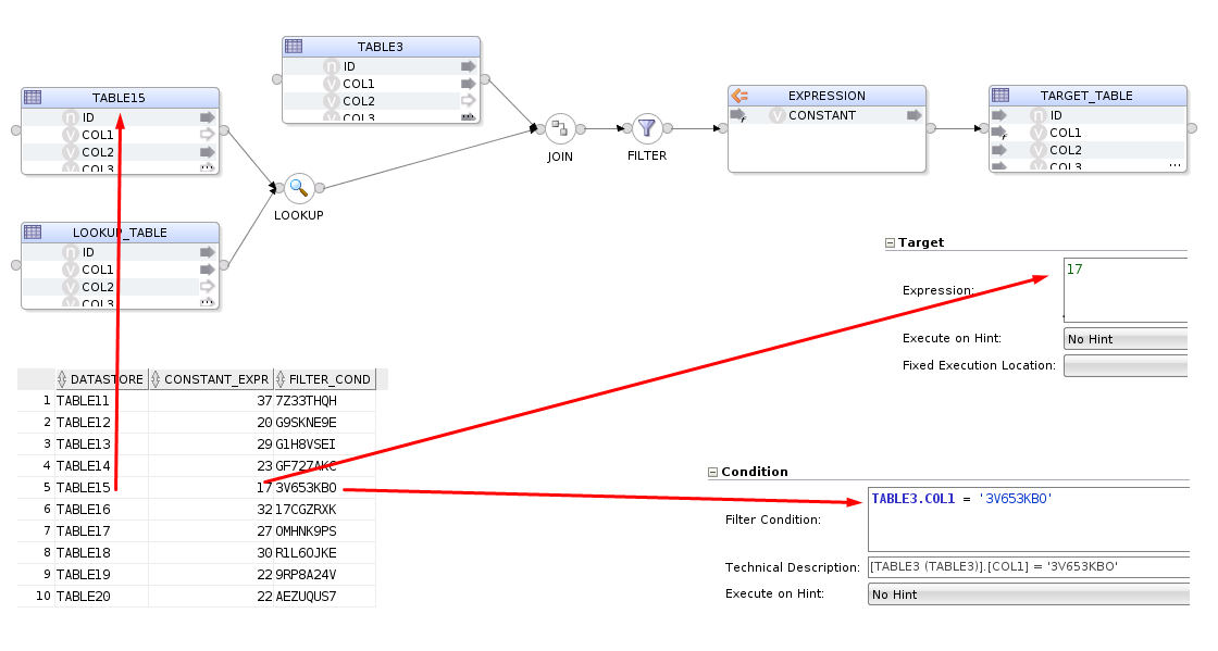
Let's take this, hand built, fictional and completely CRAZY_MAPPING as an example. (fictional and crazy in the sense that it does nothing useful, however, the flow and configuration are completely valid).

If we execute .reverse() on this mapping by calling...
mapping.reverse('MY_PROJECT', 'DEMO_FOLDER', 'CRAZY_MAPPING')
...OdiDsl will return the following output to the console. What you are seeing here is the OdiDsl required to recreate the crazy mapping above.
Connecting to the repository...

mapping.create('MY_PROJECT', 'DEMO_FOLDER', 'CRAZY_MAPPING')
    .datastores([
         ['name':'STAGING.TABLE1', 'alias':'TABLE1'],
         ['name':'STAGING.TABLE9', 'alias':'TABLE9'],
         ['name':'STAGING.TABLE3', 'alias':'TABLE3'],
         ['name':'STAGING.TABLE4', 'alias':'TABLE4'],
         ['name':'STAGING.TABLE6', 'alias':'TABLE6'],
         ['name':'STAGING.TABLE5', 'alias':'TABLE5'],
         ['name':'STAGING.TABLE7', 'alias':'TABLE7'],
         ['name':'STAGING.TABLE2', 'alias':'TABLE2'],
         ['name':'STAGING.TABLE8', 'alias':'TABLE8'],
         ['name':'STAGING.TABLE11', 'alias':'TABLE11'],
         ['name':'STAGING.TABLE12', 'alias':'TABLE12'],
         ['name':'STAGING.TABLE13', 'alias':'TABLE13'],
         ['name':'STAGING.TABLE15', 'alias':'TABLE15'],
         ['name':'STAGING.TABLE14', 'alias':'TABLE14'],
         ['name':'STAGING.TABLE16', 'alias':'TABLE16'],
         ['name':'STAGING.TABLE17', 'alias':'TABLE17'],
         ['name':'STAGING.TABLE42', 'alias':'TABLE42'],
    ])
    .select('TABLE5')
        .join('JOIN2', ['TABLE7'], [join_condition: "TABLE5.ID = TABLE7.ID" ])
        .join('JOIN3', ['TABLE6'], [join_condition: "TABLE6.ID = TABLE7.ID" ])
        .connect('TABLE14', [
                [ attr: "ID", expression: "TABLE5.ID" ],
                [ attr: "COL1", expression: "TABLE7.COL1" ],
                [ attr: "COL2", expression: "TABLE6.COL2" ],
                [ attr: "COL3", expression: "TABLE7.COL3" ],
                [ attr: "COL4", expression: "TABLE7.COL4" ],
        ])
    .select('JOIN3')
        .expr('EXPRESSION1', [attrs: [
                [ attr: "ID", expression: "TABLE6.ID * 42", datatype: "NUMERIC", size: "38", scale: "0"]]])
        .connect('TABLE15', [
                [ attr: "ID", expression: "EXPRESSION1.ID" ],
                [ attr: "COL1", expression: "", active_indicator: false ],
                [ attr: "COL2", expression: "TABLE6.COL2" ],
                [ attr: "COL3", expression: "TABLE7.COL3" ],
                [ attr: "COL4", expression: "", active_indicator: false ],
        ])
        .join('JOIN', ['TABLE14'], [join_condition: "TABLE14.ID = TABLE15.ID" ])
        .filter('FILTER2', [filter_condition: "TABLE15.COL3 != 'FOOBAR'" ])
        .connect('TABLE16', [
                [ attr: "ID", expression: "TABLE15.ID" ],
                [ attr: "COL1", expression: "TABLE15.COL1" ],
                [ attr: "COL2", expression: "TABLE14.COL2" ],
                [ attr: "COL3", expression: "TABLE14.COL3" ],
                [ attr: "COL4", expression: "TABLE14.COL4" ],
        ])
    .select('JOIN')
        .connect('TABLE17', [
                [ attr: "ID", expression: "TABLE15.ID" ],
                [ attr: "COL1", expression: "TABLE15.COL1" ],
                [ attr: "COL2", expression: "TABLE14.COL2" ],
                [ attr: "COL3", expression: "TABLE14.COL3" ],
                [ attr: "COL4", expression: "TABLE14.COL4" ],
        ])
    .select('TABLE5')
        .sort('SORT1', [sorter_condition: "TABLE5.ID, TABLE5.COL2, TABLE5.COL4" ])
        .connect('TABLE13', [
                [ attr: "ID", expression: "TABLE5.ID" ],
                [ attr: "COL1", expression: "TABLE5.COL1" ],
                [ attr: "COL2", expression: "TABLE5.COL2" ],
                [ attr: "COL3", expression: "TABLE5.COL3" ],
                [ attr: "COL4", expression: "TABLE5.COL4" ],
        ])
    .select('TABLE3')
        .filter('FILTER1', [filter_condition: "TABLE3.ID != 42" ])
    .select('TABLE4')
        .filter('FILTER', [filter_condition: "TABLE4.COL1 = 42" ])
        .lookup('LOOKUP1', 'FILTER1', [join_condition: "TABLE4.ID = TABLE3.ID AND TABLE3.COL1 = TABLE4.COL1"])
        .join('JOIN5', ['TABLE13'], [join_condition: "TABLE13.ID = TABLE3.ID" ])
        .distinct('DISTINCT_', [attrs: [
                [ attr: "COL3_1", expression: "TABLE4.COL3", datatype: "VARCHAR", size: "30"],
                [ attr: "COL4_1", expression: "TABLE4.COL4", datatype: "VARCHAR", size: "30"]]])
    .select('DISTINCT_')
        .join('JOIN4', ['EXPRESSION1'], [join_condition: "TABLE5.ID = TABLE6.COL1" ])
        .sort('SORT', [sorter_condition: "EXPRESSION1.ID" ])
        .connect('TABLE8', [
                [ attr: "ID", expression: "EXPRESSION1.ID" ],
                [ attr: "COL1", expression: "", active_indicator: false ],
                [ attr: "COL2", expression: "", active_indicator: false ],
                [ attr: "COL3", expression: "TABLE7.COL3" ],
                [ attr: "COL4", expression: "", active_indicator: false ],
        ])
        .connect('TABLE12', [
                [ attr: "ID", expression: "TABLE8.ID" ],
                [ attr: "COL1", expression: "TABLE8.COL1" ],
                [ attr: "COL2", expression: "TABLE8.COL2" ],
                [ attr: "COL3", expression: "TABLE8.COL3" ],
                [ attr: "COL4", expression: "TABLE8.COL4" ],
        ])
    .select('TABLE9')
        .expr('EXPRESSION', [attrs: [
                [ attr: "ID", expression: "TABLE9.ID *42", datatype: "NUMERIC", size: "38", scale: "0"],
                [ attr: "COL4", expression: "TABLE9.COL4 || 'FOOBAR'", datatype: "VARCHAR", size: "30"]]])
        .connect('TABLE1', [
                [ attr: "ID", expression: "EXPRESSION.ID" ],
                [ attr: "COL1", expression: "", active_indicator: false ],
                [ attr: "COL2", expression: "", active_indicator: false ],
                [ attr: "COL3", expression: "", active_indicator: false ],
                [ attr: "COL4", expression: "TABLE9.COL4" ],
        ])
        .join('JOIN1', ['TABLE2'], [join_condition: "TABLE1.ID = TABLE2.ID" ])
        .aggregate('AGGREGATE', [attrs: [
                [ attr: "ID", expression: "TABLE1.ID", datatype: "NUMERIC", size: "38", scale: "0", group_by: "YES"],
                [ attr: "COL4_1", expression: "MAX(TABLE2.COL4)", datatype: "VARCHAR", size: "30", group_by: "AUTO"]]])
        .lookup('LOOKUP', 'DISTINCT_', [join_condition: "AGGREGATE.ID = DISTINCT_.COL3_1"])
        .aggregate('AGGREGATE1', [attrs: [
                [ attr: "ID", expression: "AGGREGATE.ID", datatype: "NUMERIC", size: "38", scale: "0", group_by: "YES"],
                [ attr: "COL4_1_1", expression: "SUM(AGGREGATE.COL4_1)", datatype: "VARCHAR", size: "30", group_by: "AUTO"]]])
        .filter('FILTER3', [filter_condition: "AGGREGATE1.COL4_1_1 > 42" ])
        .connect('TABLE42', [
                [ attr: "ID", expression: "AGGREGATE1.ID" ],
        ])
    .select('AGGREGATE1')
        .join('JOIN6', ['TABLE8'], [join_condition: "AGGREGATE1.ID = TABLE8.ID" ])
        .connect('TABLE11', [
                [ attr: "ID", expression: "TABLE8.ID" ],
                [ attr: "COL1", expression: "" ],
                [ attr: "COL2", expression: "" ],
                [ attr: "COL3", expression: "TABLE8.COL3" ],
                [ attr: "COL4", expression: "TABLE8.COL4" ],
        ])
    .commit()
    .validate()
When we execute this OdiDsl code we get, you guessed it, exactly the same crazy mapping with the flow and component properties all intact.

Being able to flip between ODI studio and OdiDsl has some really nice benefits for those who like the workflow. You can start prototyping a mapping in ODI Studio, convert it to code, hack around for a bit and then reflect it all back into ODI. It's also very useful for generating a "code template" from an existing mapping. The generated code template can be modified to accept variables instead of hard coded properties, all you need then is some metadata.
Did Somebody Say Metadata ?
Metadata is the key to bulk automation. You can find metadata in all kinds of places. If you are migrating to ODI from another product then there will be a whole mass of metadata living in your current product's repository or via some kind of export routine which typically produces XML files. If you are starting a fresh ODI implementation, then there will be metadata living in your source and target systems, in data dictionaries, in excel sheets, in mapping specifications documents, all over the place really. This is the kind of metadata that can be used to feed OdiDsl.
A Quick Example of One possible Approach to Using OdiDsl With Metadata
First we build a mapping in Odi Studio, this will act as our template mapping.

We then generate the equivalent OdiDsl code using mapping.reverse('MY_PROJECT', 'DEMO_FOLDER', 'FEED_ME_METADATA'). Which gives us this code.
mapping.create('MY_PROJECT', 'DEMO_FOLDER', 'FEED_ME_METADATA')
    .datastores([
         ['name':'STAGING.TABLE1', 'alias':'LOOKUP_TABLE'],
         ['name':'STAGING.TABLE2', 'alias':'TABLE2'],
         ['name':'STAGING.TABLE3', 'alias':'TABLE3'],
         ['name':'STAGING.TABLE4', 'alias':'TARGET_TABLE'],
    ])
    .select('TABLE2')
        .lookup('LOOKUP', 'LOOKUP_TABLE', [join_condition: "TABLE2.ID = LOOKUP_TABLE.ID"])
        .join('JOIN', ['TABLE3'], [join_condition: "TABLE2.ID = TABLE3.ID" ])
        .filter('FILTER', [filter_condition: "TABLE3.COL1 = 'FILTER'" ])
        .expr('EXPRESSION', [attrs: [
                [ attr: "CONSTANT", expression: "42", datatype: "VARCHAR", size: "30"]]])
        .connect('TARGET_TABLE', [
                [ attr: "ID", expression: "LOOKUP_TABLE.ID" ],
                [ attr: "COL1", expression: "LOOKUP_TABLE.COL1 || EXPRESSION.CONSTANT" ],
                [ attr: "COL2", expression: "TABLE2.COL2" ],
                [ attr: "COL3", expression: "TABLE3.COL3" ],
                [ attr: "COL4", expression: "LOOKUP_TABLE.COL4" ],
        ])
    .commit()
    .validate()
We now need to decorate this code with some variables, these variables will act as place holders for our metadata. The metadata we are going to use is from a database table, I'm keeping it simple for the purpose of this demonstration but the approach is the same. Our metadata table has 10 rows and from these 10 rows we are going to create 10 mappings, replacing certain properties with the values from the columns.
 Remember that OdiDsl is expressed in Groovy. That means, as well as OdiDsl code, we also have access to the entire Groovy language. In the following code we are using a mixture of Groovy and OdiDsl. We are connecting to a database, grabbing our metadata and then looping over
 mapping.create(), once for each row in our metadata table. The columns in the metadata table are represented as the variables row.datastore, row.constant_expr and row.filter_cond. The code comments indicate where we are substituting these variables in place of our previously hard coded property values.
import groovy.sql.Sql

// Connect to the database and retrieve rows from the METADATA table.
def sqlConn = Sql.newInstance("jdbc:oracle:thin:@hostname:1521/pdborcl", "username", "password", "oracle.jdbc.pool.OracleDataSource")
def rows = sqlConn.rows("SELECT * FROM METADATA")
sqlConn.close()

// For each row in our METADATA table
rows.eachWithIndex() {  row, index ->

    mapping.create('MY_PROJECT', 'DEMO_FOLDER', "FEED_ME_METADATA_${index+1}") // Interpolate row number to make the mapping name unique
            .datastores([
                    ['name': 'STAGING.TABLE1', 'alias': 'LOOKUP_TABLE'],
                    ['name': "STAGING.${row.datastore}" ], // substitute in a different datastore
                    ['name': 'STAGING.TABLE3', 'alias': 'TABLE3'],
                    ['name': 'STAGING.TABLE4', 'alias': 'TARGET_TABLE'],
            ])
            .select(row.datastore)
                .lookup('LOOKUP', 'LOOKUP_TABLE', [join_condition: "${row.datastore}.ID = LOOKUP_TABLE.ID"]) // substitute in a different datastore
                .join('JOIN', ['TABLE3'], [join_condition: "${row.datastore}.ID = TABLE3.ID"]) // substitute in a different datastore
                .filter('FILTER', [filter_condition: "TABLE3.COL1 = '${row.filter_cond}'"]) // substitute in a different filter condition
                .expr('EXPRESSION', [attrs: [
                    [attr: "CONSTANT", expression: row.constant_expr, datatype: "VARCHAR", size: "30"]]]) // substitute in a different constant for the expression
                .connect('TARGET_TABLE', [
                    [attr: "ID", expression: "LOOKUP_TABLE.ID"],
                    [attr: "COL1", expression: "LOOKUP_TABLE.COL1 || EXPRESSION.CONSTANT"],
                    [attr: "COL2", expression: "${row.datastore}.COL2"], // substitute in a different datastore
                    [attr: "COL3", expression: "TABLE3.COL3"],
                    [attr: "COL4", expression: "LOOKUP_TABLE.COL4"],
                ])
            .commit()
            .validate()

}
Here is the output...
Connecting to the repository...

mapping FEED_ME_METADATA_1 created
Validation Successful
mapping FEED_ME_METADATA_2 created
Validation Successful
mapping FEED_ME_METADATA_3 created
Validation Successful
mapping FEED_ME_METADATA_4 created
Validation Successful
mapping FEED_ME_METADATA_5 created
Validation Successful
mapping FEED_ME_METADATA_6 created
Validation Successful
mapping FEED_ME_METADATA_7 created
Validation Successful
mapping FEED_ME_METADATA_8 created
Validation Successful
mapping FEED_ME_METADATA_9 created
Validation Successful
mapping FEED_ME_METADATA_10 created
Validation Successful
And here are our 10 mappings, each with it's own configuration.
 If we take a look at the
 FEED_ME_METADATA_5 mapping, we can see the metadata has been reflected into the mapping.
And that's about it. We've basically just built a mini accelerator using OdiDsl and we hardly had to write any code. The OdiDsl code was generated for us using .reverse(). All we really had to code, was the connection to the database, a loop and bit of variable substitution!
Summary
With the Rittman Mead ODI Tool kit, accelerating your ODI implementation has never be easier. If you are thinking about migrating to ODI from another product or embarking on a new ODI Project, Rittman Mead can help. For more information please get in touch.
Create Your Own DVD Plugin in 22 minutes
Introduction
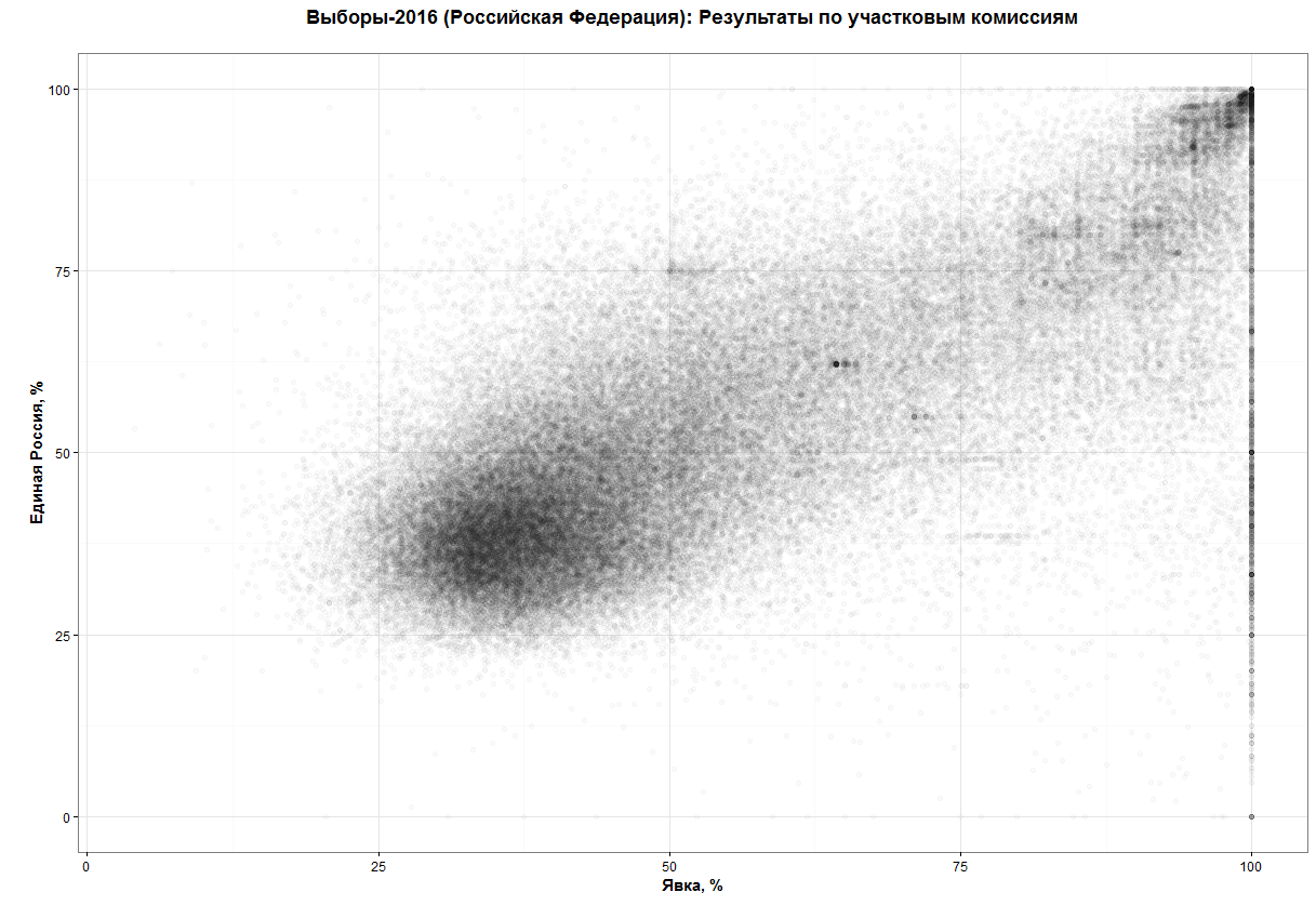
Oracle DVD played well for the task of elections data analysis. But I faced some limitations and had to curtail my use of one of my favourite charts - Scatter chart. While DVD’s implementation of it looks good, has smooth animations and really useful, it is not suitable for visualisations of huge datasets. Election dataset has about 100K election precinct data rows and if I try to plot all of them at one chart I will get something close to this. It doesn't really important what is the data, just compare how charts look like.
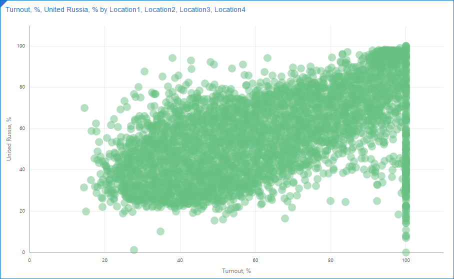
This picture can give us about zero insights. Actually, I'm not even sure if shows my 100K points. What I want to get is something like this:
 (source: https://habrahabr.ru/post/313372/)
What can I see at this chart and can't see at the vanilla one? First of all, it gives a much better understanding of points distribution other the plot. I can see a relatively dense core around coordinates [30;40] and then not so dense tail growing by both dimensions and again a small and very dense core in the top right corner.
Secondly, it not only shows dense and sparse areas but shows that there are exist a few points which have an unexplainably high concentration. Around [64;62], for example.
Luckily DVD allows me (and anyone else too) create custom plugins. That's what I'm going to show here. The plugin I'm going to do is something I'd call Minimum Viable Product. It's very, very simple and needs a lot of work to make it good and really useful.
The code I'm going to show is the simplest I can invent. It doesn't handle errors, exceptions and so on. It should be more modular. It possibly could use some optimisation. But that was done for a purpose. And the purpose is called 'simplicity'. If you want a more comprehensive sample, there is a link to the Oracle's guide in the Summary. I want to show you that writing a DVD plugin is not a rocket science. It takes less than half an hour to build your own DVD plugin.
And the clock starts now!
[0:00-5:40] Setup Environment and DVD SDK
Setup
Download and install DVD. I presume you already have it, because from my experience people who doesn't have it very rarely feel a need for its plugins. Hence I didn't include download and installation times into 22 minutes.
Create a folder to store your plugins and some Gradle-related configs and scripts. It may be any directory you like, just select your favourite place.
Next step is to define some environment variables.
- The first one is
DVDDESKTOP_SDK_HOMEand it should point to thу DVD folder. In most of the cases, it isC:\Program files\Oracle Data Visualisation Desktop. - The second variable is
PLUGIN_DEV_DIRit points to the folder you created 40 seconds ago. These two variables seem not to be absolutely necessary, but they make your life a bit easier. - And one more change to the environment before going further. Add
%DVDESKTOP_SDK_HOME%\tools\binto thePATHvariable (do you feel how your life became easier withDVDDESKTOP_SDK_HOMEalready defined so you can start using it right now?).
And the last step is to initialise our development environment. Go to the plugins directory and execute the initialization command. Open cmd window and execute:
cd %PLUGIN_DEV_DIR%
bicreateenv
This will not only initialise everything your need but create a sample plugin to explore and research.
Let's take a look at what we got. In the folder we have created before (%PLUGIN_DEV_DIR%) this command generated the following structure.
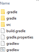
All names here are more than self-explanatory. You won't need to do anything with .gradle and gradle, and src stores all the code we will develop. Please notice that src already has sample plugin sampleviz. You may use it as a referrence for your own work.
Create First Plugin
Every plugin consists of a few parts. We don't need to create them from scratch every time. Oracle gives us a simple way of creating a new plugin. If you didn't close cmd window from previous steps execute the following:
bicreateplugin viz -id com.rittmanmead.demo -subType dataviz
Obviously, you should use your own company name for the id. The last word (demo) plus word Plugin is what user will see as a visualisation name. Obviously we can change it but not today.
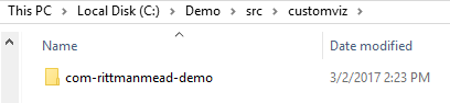
This will create a fully operational plugin. Where can we find it? You shouldn't be too surprised if I say "In src folder".
And we may test it right now. Yes, its functionality is very limited, but you didn't expect it to do something useful, right?
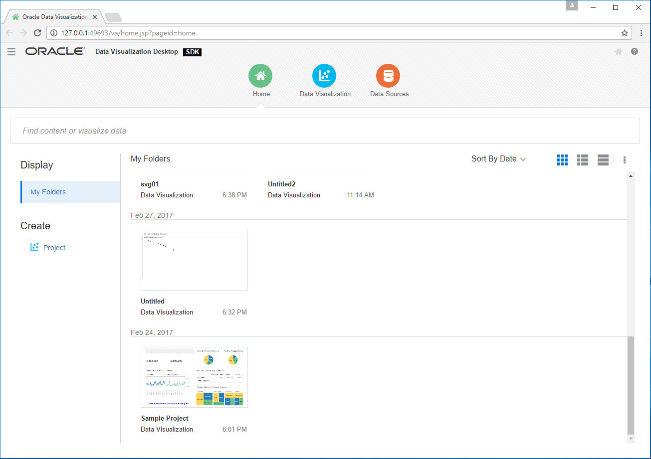
Start SDK
Now we should start Oracle DVD in SDK mode. The main difference from the normal mode is that DVD will start in the default browser. That's not a typo. DVD will start as a usual site in a browser. It's a good idea to select as the default a browser with good developer console and tools. I prefer Chrome for this task but that's not the only choice. Choose the browser you'd normally use for site development. When you finish with setting up of the default browser do:
cd %PLUGIN_DEV_DIR%
.\gradlew run
If you don't have an ultrafast computer I'd recommend you to make some tea at this point. Because the very first start will take a long time. Actually, it will consume most of the first stage time.
[5:40-6:15] Test the Plugin
We didn't start changing the first plugin yet, so I expect everything to be OK at this point. But anyway it's a good idea to test everything. I think we can afford 30-40 seconds for this.
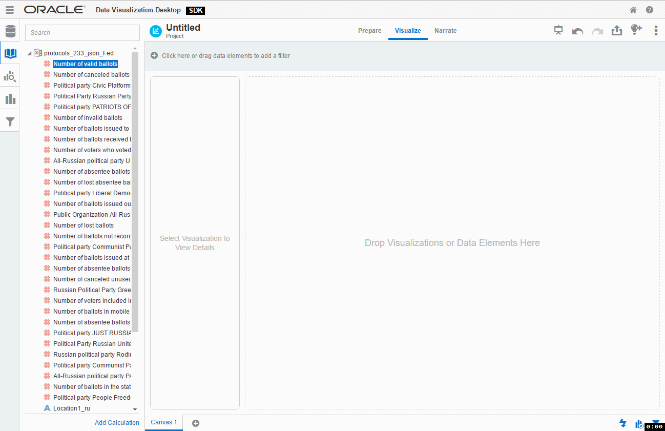
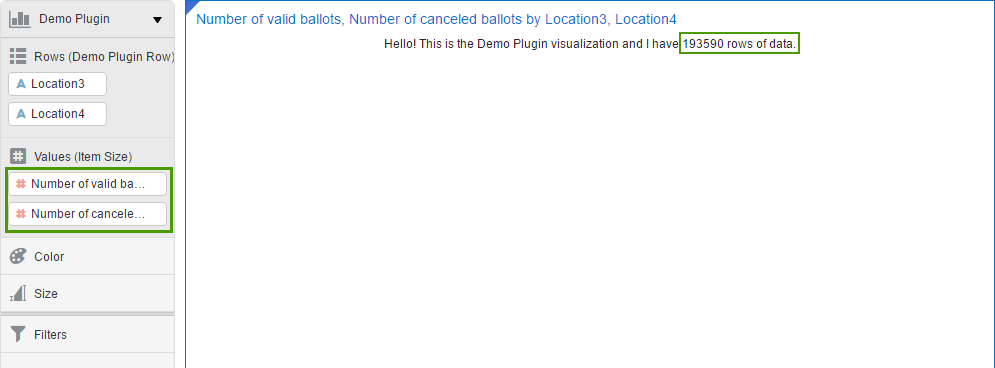
And again I assume you know how to use DVD and don't need a step-by-step guide on creating a simple visualisation. Just create a new project, select any data source, go to Visualisations, find your plugin and add it. You may even add some data to the plugin and it will show how many rows your data has. I think that's a good place to start from.
[6:15-22:00] Add Functions
Change parameters
If you didn't skip testing phase and played with this new toy for a while you may have noticed two things we need to change right now. First, for a chosen type of visualisation, I need that my plugin can accept two measures. You possibly noticed that I was unable to add Number of cancelled ballots as a second measure. By default a plugin accepts not more than one (zero or one). Luckily it can be changed very easily.
We can find all parameter about measures, rows, columns etc inside of extensions folder. In this case it is %PLUGIN_DEV_DIR%\customviz\com-rittmanemad-demo\extensions. Here we can find two folders. The first one is oracle.bi.tech.pluginVisualizationDataHandlerand it has only one file com.rittmanemad.demo.visualizationDataHandler.JSON. This file allows us to define which types of input data our plugin has (measures, columns, rows, colour etc.), what are their types (measures/dimensions), which is the default one and so on.
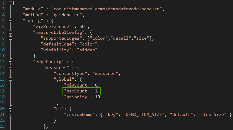 Here we should change
 maxCount to 2. This will allow us to add more than one measure to our visualisation.
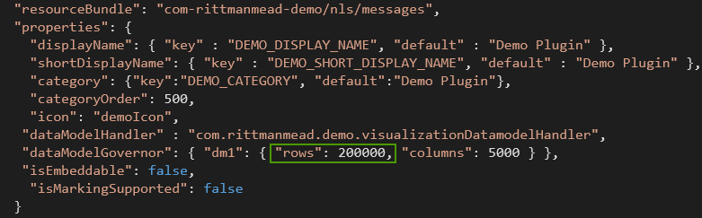
The second thing I want to change is the number of data points. Elections dataset has data about 100K precinct commissions. And DVD's default is 10K. We can change this value in the second configuration file from extensions folder. Its name is oracle.bi.tech.Visualization. There is again only one JSON file com.rittmanmead.demo.json. We need to change rows to 200000.
Why 200000 if I need only 100000 points? Well, it's about how data will be passed to our code. Every measure is a separate row, so I need 100K points with 2 measures each and that gives me 200000 rows. It looks like right now that's the only way to have more than one measure in a plugin (at least it's my best knowledge for DVD 12.2.2.2.0-20170208162627).
Note. I could change here some things like plugin name, input data types shown to user and so on but my aim is simplicity.
Now we should restart DVD SDK in order to use new parameters.
Write code
For my custom scatter chart I'm going to use d3js JavaScript library. It will allow me to concentrate more on logic and less on HTML manipulation. To add it to my plugin I should add a couple of strings in the beginning of my code.
Before:
define(['jquery',
        'obitech-framework/jsx',
        'obitech-report/datavisualization',
        'obitech-reportservices/datamodelshapes',
        'obitech-reportservices/events',
        'obitech-appservices/logger',
        'ojL10n!com-rittmanmead-demo/nls/messages',
        'obitech-framework/messageformat',
        'css!com-rittmanmead-demo/demostyles'],
        function($,
                 jsx,
                 dataviz,
                 datamodelshapes,
                 events,
                 logger,
                 messages) {
After (I added two lines starting with d3):
define(['jquery',
        'obitech-framework/jsx',
        'obitech-report/datavisualization',
        'obitech-reportservices/datamodelshapes',
        'obitech-reportservices/events',
        'obitech-appservices/logger',
      'd3js',
        'ojL10n!com-rm-domoViz/nls/messages',
        'obitech-framework/messageformat',
        'css!com-rittmanmead-demo/demostyles'],
        function($,
                 jsx,
                 dataviz,
                 datamodelshapes,
                 events,
                 logger,
               d3,
                 messages) {
That's all. Now I can use d3js magic. And that's cool.
OK, it's time to make our plugin do something more useful than a simple counting of rows. All plugin code is in demo.js file and the main procedure is render. It is called every time DVD needs to update the visualisation. The initial version of this function is really small. Without comments there are only four rows. It retrieves data, counts rows, then finds a container to write and writes a message.
Demo.prototype.render = function(oTransientRenderingContext) {
      // Note: all events will be received after initialize and start complete.  We may get other events
      // such as 'resize' before the render, i.e. this might not be the first event.

      // Retrieve the data object for this visualization
  var oDataLayout = oTransientRenderingContext.get(dataviz.DataContextProperty.DATA_LAYOUT);

      // Determine the number of records available for rendering on ROW
      // Because we specified that Category should be placed on ROW in the data model handler,
      // this returns the number of rows for the data in Category.
  var nRows = oDataLayout.getEdgeExtent(datamodelshapes.Physical.ROW);

      // Retrieve the root container for our visualization.  This is provided by the framework.  It may not be deleted
      // but may be used to render.
  var elContainer = this.getContainerElem();
  $(elContainer).html(messages.TEXT_MESSAGE.format("Demo Plugin", "" + nRows));
};
First of all, I need to know the actual size of the plotting area. I simply added that after var elContainer = this.getContainerElem();:
  [...]
  var elContainer = this.getContainerElem();

  //container dimensions
  var nWidth = $(elContainer).width();
  var nHeight = $(elContainer).height();
  [...]
The template plugin has code for pulling the data into the script (oDataLayout variable). But for my scatter plot, I need to put this data into an array and find the minimum and the maximum value for both measures. This part of the code is my least favourite one. It looks like currently we can't make two separate measures in a custom viz (or at least I can't find the solution), therefore instead of two nice separate measures, I have them as different rows. Like:
| ... | ... | ... |
| PEC #1 | Turnout,% | 34,8% |
| PEC #1 | United Russia,% | 44,3% |
| PEC #2 | Turnout,% | 62,1% |
| PEC #2 | United Russia,% | 54,2% |
| PEC #3 | Turnout,% | 25,9% |
| PEC #3 | United Russia,% | 33,2% |
| ... | ... | ... |
I really hope that any solution for this will be found. So far I just put even and odd rows into X ad Y coordinates. At the same time, I determine minimum and maximum values for both axes.
  //temporary measure
  var tmp_measure;

  //current measure
  var cur_measure;

  var vMinimax=[Number.MAX_VALUE, Number.MIN_VALUE];
  var hMinimax=[Number.MAX_VALUE, Number.MIN_VALUE];

  for(var i=0;i<nRows;i++){

    if(i%2==1){
      cur_measure=Number(oDataLayout.getValue(datamodelshapes.Physical.DATA, i, 0, false));
      vMinimax[0]=Math.min(vMinimax[0], cur_measure);
      vMinimax[1]=Math.max(vMinimax[1], cur_measure);
      points.push([cur_measure,tmp_measure]);
    }
    else{
      tmp_measure=Number(oDataLayout.getValue(datamodelshapes.Physical.DATA, i, 0, false));
      hMinimax[0]=Math.min(hMinimax[0], tmp_measure);
      hMinimax[1]=Math.max(hMinimax[1], tmp_measure);
    }
  }
The next part of the code is about handling multiple calls. I should handle things like changing measures or dimensions. I simply delete the old chart and create a new empty one.
  var oSVG;

  //Delete old chart if exists
  d3.select("#DemoViz").remove();

  //Create new SVG with id=DemoViz
  oSVG=d3.select(elContainer).append("svg");
  oSVG.attr("id","DemoViz");

  //Set plot area size
  oSVG=oSVG
       .attr("width", nWidth)
       .attr("height", nHeight)
       .append("g");
Now I have an array with data. I have a prepared SVG plot for drawing. And I have no reason not to combine all this into a chart.
  //Compute scaling factors
  var hStep=(nWidth-40)/(hMinimax[1]-hMinimax[0]);
  var vStep=(nHeight-40)/(vMinimax[1]-vMinimax[0]);

  //Draw
  oSVG.selectAll("rect")
      .data(points)
      .enter()
      .append("rect")
      .attr("x", function(d) {return 20+d[1]*hStep;})
      .attr("y", function(d) {return nHeight-(20+d[0]*vStep);})
      .attr("height",1).attr("width",1)
      .attr('fill-opacity', 0.3);
What I should mention here is opacity. If its value is too high (almost no opacity) the chart looks like this:
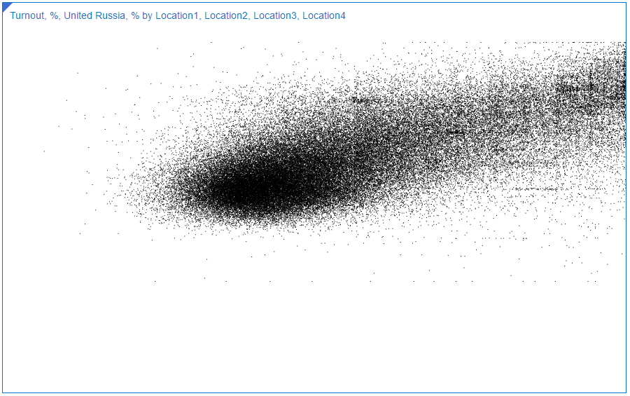
If I make dots more opaque, the chart looks (and works) better. This is how it looks like with fill-opacity=0.3.
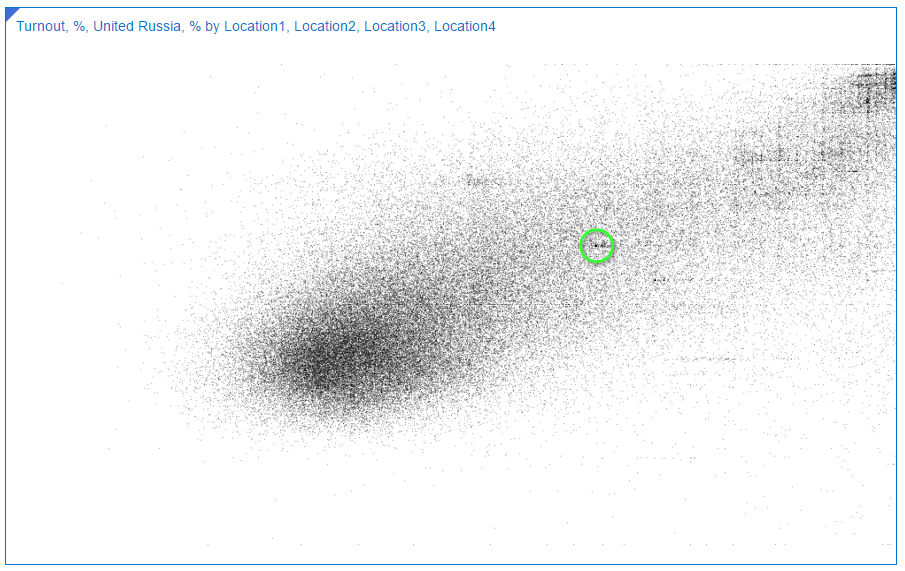 Look at the black point in the middle. It's there because a lot of commissions has exactly the same values for both measures. That's how we could find Saratov region anomaly.
[22:00-] Summary and TODOs
This shows how we may enhance Oracle DVD with our own visualisation. Yes, it's really, really, really simple. And it needs a lot of work in order to make it more useful. First of all, we should make it more reliable. This realisation doesn't test input parameters for correctness. And we also need to add interactivity. The chart should be zoomable and selectable. It should work as a filter. It should react to resize. It needs visible axes. And so on. But we can create it in less than a half of hour and I think as a first step it works well. I hope you don't afraid of making your own plugins now.
If you need more complex sample, take a look at the Oracle's tutorial. It covers some of these TODOs.
A Case for Essbase and Oracle Data Visualization
So it’s the end of the month, or maybe even the end of the quarter. And you’ve found yourself faced, yet again, with the task of pulling whatever data will be needed to produce the usual standardized budgetary and / or finance reports. You’re dreading this as it will probably eat up most of your day just getting the data you need, combing through it to find the metrics you need, and plugging them into your monumentally complicated custom spreadsheet, only to find the numbers are, well, off.

Enter Data Visualization (DV), and its lightweight brother application, Data Visualization Desktop (DVD). My bud at RM, Matt Walding, already did a pretty great post on some of the cursory features of DVD, covering a lot of the important how-tos and what’s whats. So check that out if you need a bit of a walkthrough. Both of these great tools tout that you can go from zero to analysis pretty darn quick, and from the extensive testing and prodding we’ve done with both DV and DVD, this claim is accurate. Now how does this help us, however, in the previous scenario? Well, IT processes being what they are in a lot of mid to large size companies, getting the data we need, to do the crunching we need to do, can be quite the monumental task, let alone the correct data. So when we get it, we are going to want a solution that can take us from zero to report, pretty darn quick.
If you’re the one stuck with doing the crunching, and then providing the subsequent results, your solution or workflow probably resembles one of the following:
Scenario 1

Emailed a spreadsheet with a ton of rows. Download the csv/xlsx and then crunch the rows into something that you can force into a super spreadsheet that has a ton of moving pieces just waiting to throw an error.
Scenario 2

You have access to Essbase, which stays pretty fresh, especially as reporting time draws nigh. You connect to Smartview and extract what you need for your report. See scenario 1.
Scenario 3

You have OBIEE that you depend on for data dumps, and then just export whatever you need. See scenario 1.
While there are no doubt variations on these themes, the bigger picture here is that between the time you receive your dataset and the final report, there are likely a few iterations of said final report. Maybe you’re having to make corrections to your Excel templates, perhaps the numbers on your sheet just aren’t jiving. Whatever the case may be, this part of the process is often the one that can be the most demanding of your time, not to mention the most headache inducing. So what’s the point of my schpeal? Well, wouldn’t it be nice to expedite this part of the whole thing? Let’s take a look at how we can do just that with both Data Visualization in OBIEE and Data Visualization Desktop.
Data Visualization
With DV, we can simply access any of our existing OBIEE subject areas to quickly create a basic pivot table. Right away you can see the profound time savings garnered by using DV. What's more, you don't need to feel forced into managing OBIEE on premises, as DV is also part of BICS (Business Intelligence Cloud Service) and DVCS (Data Visualization Cloud Service).

Even if you have Smartview, and can do more or less the same thing, what if you wanted to delegate some of the tedium involved in manually crunching all those rows? You could simply hand off an export to another analyst, and have them plug it right into their own instance of Data Visualization Desktop, which, might I add, comes with your purchase of the DV license. This also, however, leads down the slippery slope into siloing off your department. This approach is essentially doing that, however kept under the quarantine that is DVD, as this blog is touting, and keeping the data with which you are working consistent, you shouldn't be able to do too much damage. The point I'm trying to make is that everything about using DV and DVD as your sort of report crafting and proofing mediums, is super-fluid and smooth. The process from source system to report and over and over again, is super-seamless. Even if I didn't have direct access to the data source I needed, and had to rely on emailed data dumps or other, I can simply upload that sheet right into DV, assign some data types, and get to work. I can even add dynamic filters to the analysis by simply dragging and dropping a column to the filters area. If you're feeling adventurous, you could also display these tables on a dashboard, that perhaps your department looks at to proof them and share in the pleasurable experience that is concocting period-end reporting.

![]()

Data Visualization Desktop
Right now, DVD is only out for Windows (with a version for the Mac on the roadmap), which is mostly ok, as most every medium to large size company I have worked with employs Windows as their go-to OS. An analyst can install the program on their desktop machine and be ready to plug away in under 10 minutes. We can take the example spreadsheet above that we dumped out of VA and create our own version of the report right in DVD. One better, we can also blend it with any other source DVD can connect to. This feature, especially, can save lots of time when trying to get your numbers just right for sign off.
Looks Just Like DV

Acts Just Like DV


And hold the phone! There's even a native Essbase connector!


Actually One Better Than DV!
Speaking of connectors, check out the rest of the list, as well as the custom data flow functionality, which allows you to construct and save in-app data transformations to be invoked again, and again, and again...

Summary
Flexibility is the name of the game with DV and DVD. So sure, while it isn't the ideal tool for creating precisely formatted financial statements for SEC submission, it sure beats massaging and munging all that data in Excel. And once we're happy with our numbers, either by sharing our reports on a dashboard, or export, we can go ahead and plug our numbers right into whatever tool we are going to use to produce the final product. We've covered a couple of really good concepts, so let's just do a bit of a wrap up to make everything a bit more cohesive.
We can pull data into Data Visualization from OBIEE, from a spreadsheet, or even mash up the two to handle any inconsistencies that may exist at month's/quarter's end. Note that we can also use Smartview to pull directly to Excel. Note that you will be unable to use the OLAP capabilities of Essbase / Essbase in OBIEE, as the data will presented in DV and DVD as flattened hierarchies.
We can share reports in Data Visualization with other analysts or approvers via a dashboard (note that this is not a supported feature, but something that requires only a 'bit' of a hack) or PDF, or hand off our exported data set for further work. This can be to another person using DV or DVD.
Data Visualization Desktop can connect directly to our Essbase source or utilize a data dump from DV / OBIEE to do further work and analysis on the data set. We can also connect DVD to OBIEE, as posted here, in order to extract an analysis from the web catalog. This will at least save us the step of dumping / emailing the report.
All of this app-to-app compatability encourages a sustainable, functional, and fluid reporting environment (warning: data silos!), especially for those who are unfamiliar with the ins and outs of Essbase and / or working with OBIEE.