Category Archives: Rittman Mead
Democratize Data Science with Oracle Analytics Cloud - Data Analysis and Machine Learning
Welcome back! In my previous Post, I described how the democratization of Data Science is a hot topic in the analytical industry. We then explored how Oracle Analytics Cloud can act as an enabler for the transformation from Business Analyst to Data Scientist and covered the first steps in a Data Science project: problem definition, data connection & cleaning. In today's post, we'll cover the second part of the path: from the data transformation and enrichment, the analysis, the machine learning model training and evaluation. Let's Start!
Step #3: Transform & Enrich
In the previous post, we understood how to clean data in order to handle wrong values, outliers, perform aggregation, feature scaling and divide our dataset between train and test. Cleaning the data, however, is only the first step in data processing, and should be followed by what in Data Science is called Feature Engineering.
Feature Engineering is a fancy name to call what in ETL terms we always called data transformation, we take a set of columns in input and we apply transformation rules to create new columns. The aim of Feature Engineering is to create good predictors for the following machine learning model. Feature Engineering is a bit of black art and to achieve excellent results requires a deep understanding of the ML Model we intend to use. However, most of the basic transformations are actually driven by domain knowledge: we should create new columns that we think will improve the problem explanation. Let's see some examples:
- If we're planning to predict the Taxi Fare in New York between any two given points and we have source and destination, a good predictor for the fare probably would be the Euclidean distance between the two.
- If we have Day/Month/Year on separate columns, we may want to condense the information in a unique column containing the Date
- In case our dataset contains location names (Cities, Regions, Countries) we may want to geo-tag those properly with ZIP codes or ISO Codes.
- If we have personal information like Credit Cards details or Person Name, we may want to decide to obfuscate or extract features like the person's sex from the name (on this topic please check the blog post about GDPR and ML from Brendan Tierney).
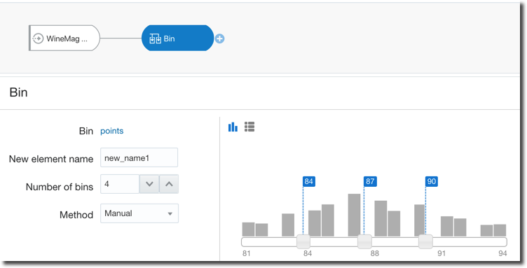
- If we have continuous values like the person's age, do we think there is much difference between a 35, 36 or 37 year-old person? If not we should think about binning them in the same category.
- Most Machine Learning Models can't cope with categorical data, thus we need to transform them to numbers (aka encoding). The standard process, when no ordering exists between the labels, is to create a new column for each value and mark the rows with
1/0accordingly.
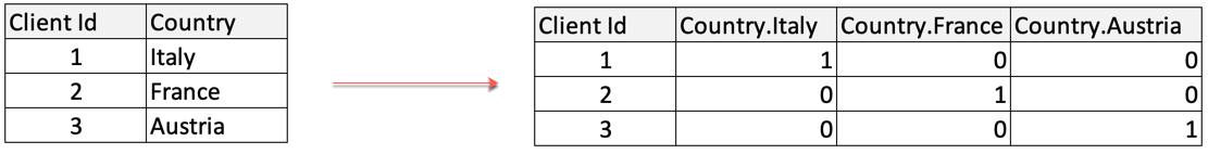
Oracle Analytics Cloud again covers all the above cases with two tools: Euclidean distance, generic data transformation like data condensation and binning are standard steps of the Dataflow component. We only need to set the correct parameters or write simple SQL-like statements. Moreover, for binning, there are options to do it manually as well as automatically providing equal-width and equal-height bins therefore taking out the manual labour and related BIAS.
On the other side the geo-tagging, data obfuscation, automatic feature extraction (like person's sex based on name) is something that with most of the other tools needs to be resolved by hand, with complex SQL statements or dedicated Machine Learning efforts.
OAC again does a great job during the Data Preparation Recommendation step: after defining a data source, OAC will scan column names and values in order to find interesting features and propose some recommendations like geo-tagging, obfuscation, data splitting (e.g. Full Name split into First and Last Name) etc.
The accepted recommendations will be added to a Data Preparation Script that can be automatically applied when updating our dataset.
Step #4: Data Analysis
Data Analysis is declared as Step #4 however since the Data Transformation and Enrichment phase we started a circular flow in order to optimize our predictive model output.
The analysis is a crucial step for any Data Science project; in R or Python one of the first steps is to check dataset head() that will show a first overview of the data like the below
OAC does a similar job with the Metadata Overview where we can see for each column the name, type and sample values as well as the Attribute/Metric definition and associated aggregation than we can then change later on.
Analysing Data is always a complex task and is where the expert eye of a data scientist makes the difference. OAC, however, can help with the excellent Explain feature. As described in the previous post, by right clicking on any column in the dataset and selecting Explain, OAC will start calculating statistics and metrics related to the column and display the findings in graphs that we can incorporate in the Data Visualization project.
Even more, there are additional tabs in the Explain window that provide Key Drivers, Segments and Anomalies.
- Key Drivers provides the statistically significant drivers for the column we are examining.
- Segments shows hidden groups in the dataset that can predict outcomes in the column
- Anomalies does an outlier detection, showing which are corner cases in our dataset
Some Data Science projects could already end here. If the objective was to find insights, anomalies or particular segments in our dataset, Explain already provides that information in a clear and reusable format. We can add the necessary visualization to a Project and create a story with the Narrate option.
If on the other side, our scope is to build a predictive model, then it's time to tackle the next phase: Model Training & Evaluation.
Step #5: Train & Evaluate
Exciting: now it's time to tackle Machine Learning! The first thing to do is to understand what type of problem we are trying to solve. OAC allows us to solve problems in the following categories:
- Supervised when we have a history of the problem's solution and we want to predict future outcomes, we can then identify two subcategories
- Regression when we are trying to predict a continuous numerical value
- Classification when we are trying to assign every sample to a category out of two or more
- Unsupervised when we don't have a history of the solution, but we ask the ML tool to help us understanding the dataset.
- Clustering when we try to label our dataset in categories based on similarity.
OAC provides two different ways to apply Machine Learning on a dataset: On the Fly or via DataFlows. The On the Fly method is provided directly in the data visualization: when we create any chart, OAC provides the option to add Clusters, Outliers, Trend and Forecast Lines.
When adding one of the Analytics, we have some control over the behaviour of the predictive model. For the clustering image above we can decide which algorithm to implement (between K-means and Hierarchical Clustering), the number of clusters and the trellis scope in case we visualize multiple scatterplots, one for each value of a dimension.
Applying Machine Learning models on the fly is very useful and could provide some great insights, however, it suffers from a limitation: the columns analysed by the model are only the ones included in the visualization, we have no control over other columns we may want to add to the model to increase predictions accuracy.
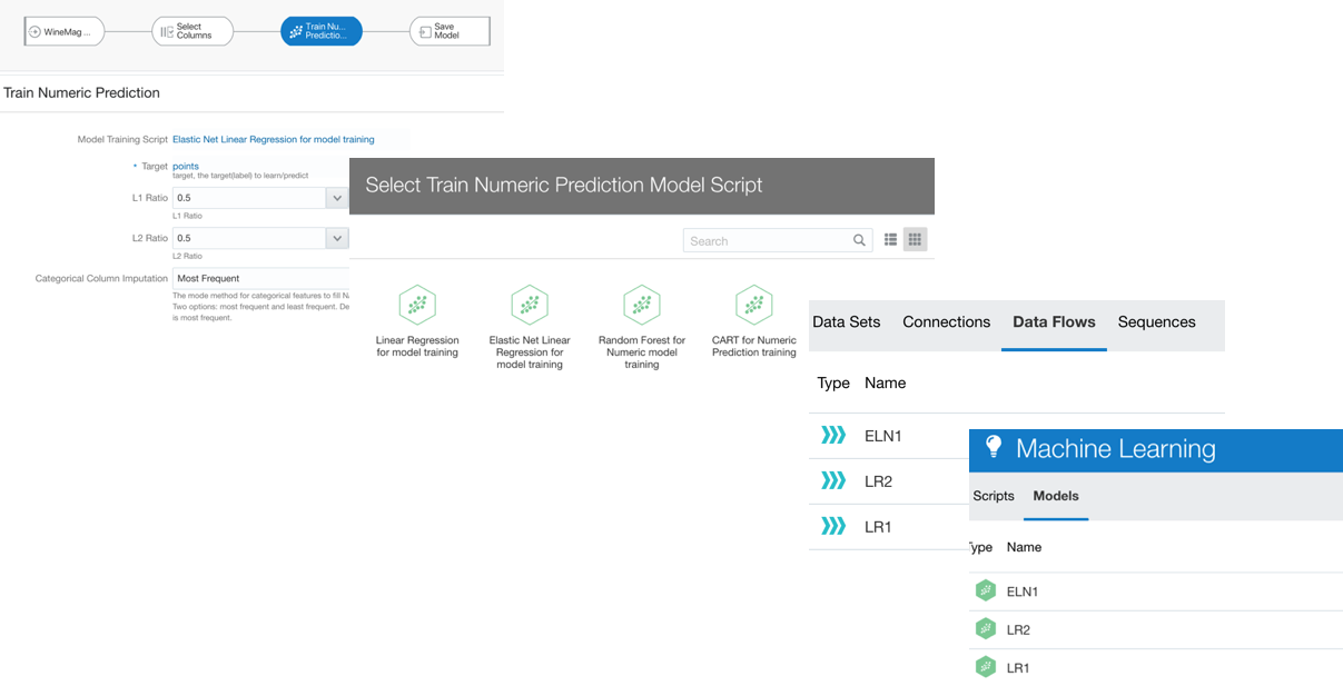
If we want to have granular control over columns, algorithm and parameters to use, OAC provides the Train Model step in the DataFlow component.
As described above OAC provides the option to solve Regression problems via Numeric Prediction, apply Binary or Multi-Classifier for Classification, and Clustering. There is also an option to train Custom Models which can be scripted by a Data Scientist, wrapped in XML tags and included in OAC (more about this topic in a later post).
Once we've selected the class of problem we're aiming to solve, OAC lets us select which Model to train between various prebuilt ones. After selecting the model, we need to identify which is the target column (for Supervised ML classes) and fix the parameters. Note the Train Partition Percent providing an automated way to split the dataset in train/test and Categorical/Numerical Column Imputation to handle the missing values. As part of this process, the encoding for categorical data is executed.
... But which Model should we use? What parameters should we pick? One lesson I got from my knowledge of Machine Learning is that there is no golden model and parameters set to solve all problems. Data Scientist will try to use different models, compare them and tune parameters based on experimentation (aka trial and error).
OAC allows us to create an initial Dataflow, select a model, set the parameters then save the Dataflow and model output. Then restart by opening the Dataflow changing the model or the parameters and storing the artefacts with different names to compare them.
After creating one or more Models, it's time to evaluate them, on OAC we can select a Model and Click on Inspect. In the Overview tab, Inspect shows the model description and properties. Far more interesting is the Quality tab which provides a set of Model scoring metrics based on the test dataset created following the Train Partition Percent parameter. In case of a Numeric Prediction problem, the Quality tab will show for each model quality metrics like the Root Mean Squared Error. OAC will provide similar metrics no matter which ML algorithm you're implementing, making the analysis and comparison easy.
In the case of Classification, the Quality Tab will show the confusion matrix together with some pre-calculated metrics like Precision, Recall etc.
The model selection then becomes an optimization problem for the metric (or set of) we picked during the problem definition (see TEP in the previous post). After trying several models, parameters, features, we'll then choose the model that minimizes the error (or increase the accuracy) of our prediction.
Note: as part of the model training, it's very important to select which columns will be used for the prediction. A blind option is to use all columns but adding irrelevant columns isn't going to provide better results and, for big or wide (huge number of columns) datasets, it becomes computationally very expensive. As written before, the Explain function provides the list of columns that represent statistically significant predictors. The columns listed there should represent the basics of the model training.
Ok, part II done, we saw how to perform Feature Engineering and Model Training and Evaluation, check my next post for the final piece of the Data Science journey: Predictions and final considerations!
Announcing The Kafka Pilot with Rittman Mead
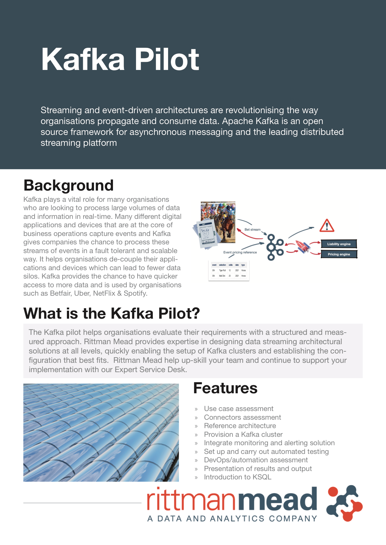
Rittman Mead is today pleased to announce the launch of it's Kafka Pilot service, focusing on engaging with companies to help fully assess the capabilities of Apache Kafka for event streaming use cases with both a technical and business focus.
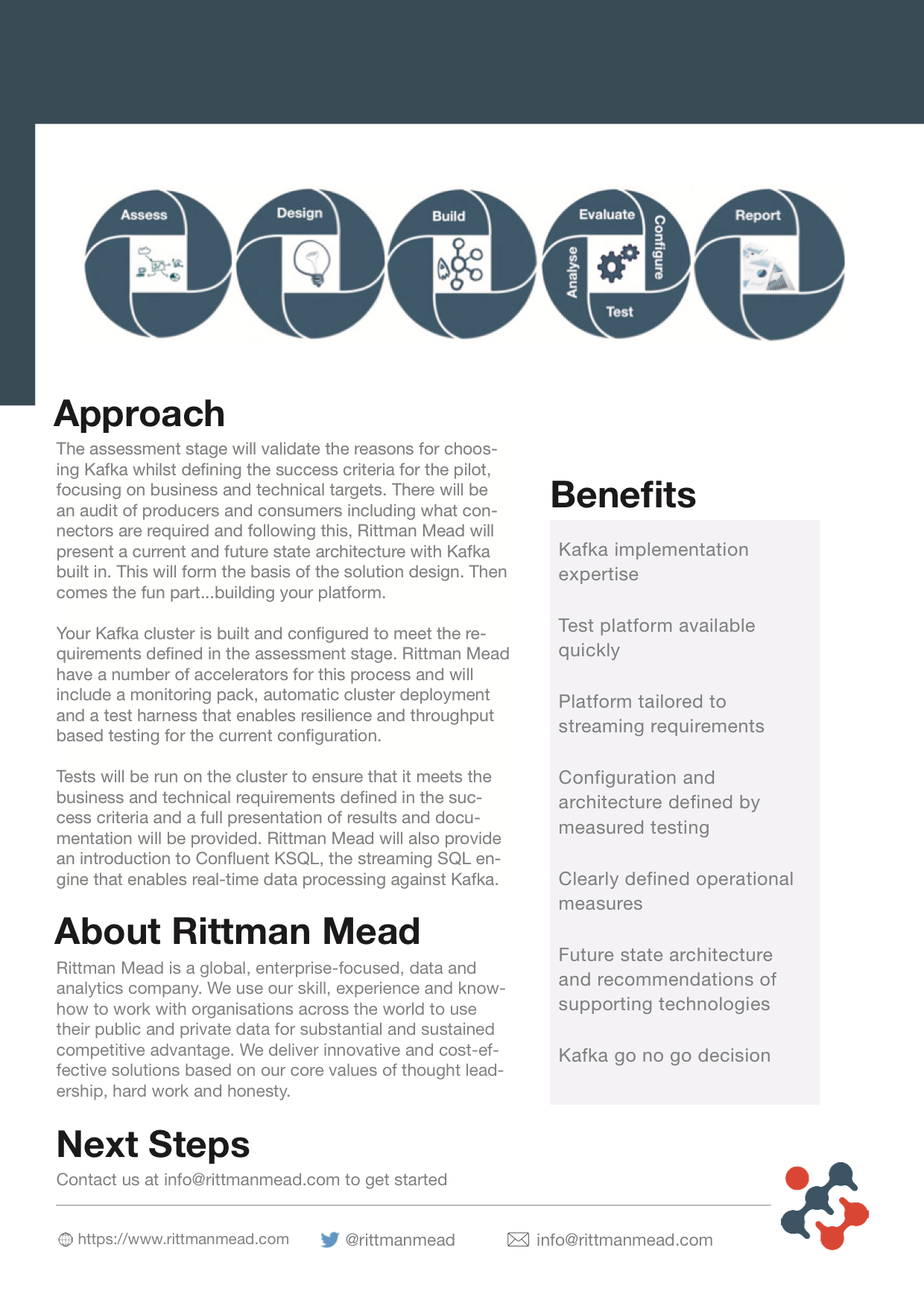
Our 30 day Kafka Pilot includes:
- A comprehensive assessment of your use cases for event streaming and Kafka
- A full assessment of connectors
- Provides a transformation from your current state to future state architecture
- Delivers your first Kafka platform with end-to-end tests built in to assess success criteria
- Introduction to KSQL
- A fully comprehensive output document detailing outcomes of the pilot, future state architecture featuring Kafka, installation & configuration details based on the platform and a roadmap for building towards a production ready platform
Kafka plays a vital role for many organisations who are looking to process large volumes of data and information in real-time. Many different digital applications and devices that are at the core of business operations capture events and Kafka gives companies the chance to process these streams of events in a fault tolerant and scalable way. It helps organisations de-couple their applications and devices which can lead to fewer data silos. Kafka provides the chance to have quicker access to more data and is used by organisations such as Betfair, Uber, NetFlix & Spotify.
Rittman Mead have written a number of blogs on the uses of Kafka ranging from using Kafka to analyse data in Scala and Spark to real-time Sailing Yacht performance. These can be read here
To find out more information about our Kafka Pilot, please read our data sheet below 👇🏼
If you'd like to discuss how event streaming and Kafka may fit into your organisation, applications and data platform please contact [email protected]
Spark Streaming and Kafka - Creating a New Kafka Connector
More Kafka and Spark, please!
Hello, world!
Having joined Rittman Mead more than 6 years ago, the time has come for my first blog post. Let me start by standing on the shoulders of blogging giants, revisiting Robin's old blog post Getting Started with Spark Streaming, Python, and Kafka.
The blog post was very popular, touching on the subjects of Big Data and Data Streaming. To put my own twist on it, I decided to:
- not use Twitter as my data source, because there surely must be other interesting data sources out there,
- use Scala, my favourite programming language, to see how different the experience is from using Python.
Why Scala?
Scala is admittedly more challenging to master than Python. However, because Scala compiles into Java bytecode, it can be used pretty much anywhere where Java is being used. And Java is being used everywhere. Python is arguably even more widely used than Java, however it remains a dynamically typed scripting language that is easy to write in but can be hard to debug.
Is there a case for using Scala instead of Python for the job? Both Spark and Kafka were written in Scala (and Java), hence they should get on like a house on fire, I thought. Well, we are about to find out.
My data source: OpenWeatherMap
When it comes to finding sample data sources for data analysis, the selection out there is amazing. At the time of this writing, Kaggle offers freely available 14,470 datasets, many of them in easy-to-digest formats like CSV and JSON. However, when it comes to real-time sample data streams, the selection is quite limited. Twitter is usually the go-to choice - easily accessible and well documented. Too bad I decided not to use Twitter as my source.
Another alternative is the Wikipedia Recent changes stream. Although in the stream schema there are a few values that would be interesting to analyse, overall this stream is more boring than it sounds - the text changes themselves are not included.
Fortunately, I came across the OpenWeatherMap real-time weather data website. They have a free API tier, which is limited to 1 request per second, which is quite enough for tracking changes in weather. Their different API schemas return plenty of numeric and textual data, all interesting for analysis. The APIs work in a very standard way - first you apply for an API key. With the key you can query the API with a simple HTTP GET request (Apply for your own API key instead of using the sample one - it is easy.):
This request
https://samples.openweathermap.org/data/2.5/weather?q=London,uk&appid=b6907d289e10d714a6e88b30761fae22
gives the following result:
{
  "coord": {"lon":-0.13,"lat":51.51},
  "weather":[
    {"id":300,"main":"Drizzle","description":"light intensity drizzle","icon":"09d"}
  ],
  "base":"stations",
  "main": {"temp":280.32,"pressure":1012,"humidity":81,"temp_min":279.15,"temp_max":281.15},
  "visibility":10000,
  "wind": {"speed":4.1,"deg":80},
  "clouds": {"all":90},
  "dt":1485789600,
  "sys": {"type":1,"id":5091,"message":0.0103,"country":"GB","sunrise":1485762037,"sunset":1485794875},
  "id":2643743,
  "name":"London",
  "cod":200
}
Getting data into Kafka - considering the options
There are several options for getting your data into a Kafka topic. If the data will be produced by your application, you should use the Kafka Producer Java API. You can also develop Kafka Producers in .Net (usually C#), C, C++, Python, Go. The Java API can be used by any programming language that compiles to Java bytecode, including Scala. Moreover, there are Scala wrappers for the Java API: skafka by Evolution Gaming and Scala Kafka Client by cakesolutions.
OpenWeatherMap is not my application and what I need is integration between its API and Kafka. I could cheat and implement a program that would consume OpenWeatherMap's records and produce records for Kafka. The right way of doing that however is by using Kafka Source connectors, for which there is an API: the Connect API. Unlike the Producers, which can be written in many programming languages, for the Connectors I could only find a Java API. I could not find any nice Scala wrappers for it. On the upside, the Confluent's Connector Developer Guide is excellent, rich in detail though not quite a step-by-step cookbook.
However, before we decide to develop our own Kafka connector, we must check for existing connectors. The first place to go is Confluent Hub. There are quite a few connectors there, complete with installation instructions, ranging from connectors for particular environments like Salesforce, SAP, IRC, Twitter to ones integrating with databases like MS SQL, Cassandra. There is also a connector for HDFS and a generic JDBC connector. Is there one for HTTP integration? Looks like we are in luck: there is one! However, this connector turns out to be a Sink connector.
Ah, yes, I should have mentioned - there are two flavours of Kafka Connectors: the Kafka-inbound are called Source Connectors and the Kafka-outbound are Sink Connectors. And the HTTP connector in Confluent Hub is Sink only.
Googling for Kafka HTTP Source Connectors gives few interesting results. The best I could find was Pegerto's Kafka Connect HTTP Source Connector. Contrary to what the repository name suggests, the implementation is quite domain-specific, for extracting Stock prices from particular web sites and has very little error handling. Searching Scaladex for 'Kafka connector' does yield quite a few results but nothing for http. However, there I found Agoda's nice and simple Source JDBC connector (though for a very old version of Kafka), written in Scala. (Do not use this connector for JDBC sources, instead use the one by Confluent.) I can use this as an example to implement my own.
Creating a custom Kafka Source Connector
The best place to start when implementing your own Source Connector is the Confluent Connector Development Guide. The guide uses JDBC as an example. Our source is a HTTP API so early on we must establish if our data source is partitioned, do we need to manage offsets for it and what is the schema going to look like.
Partitions
Is our data source partitioned? A partition is a division of source records that usually depends on the source medium. For example, if we are reading our data from CSV files, we can consider the different CSV files to be a natural partition of our source data. Another example of partitioning could be database tables. But in both cases the best partitioning approach depends on the data being gathered and its usage. In our case, there is only one API URL and we are only ever requesting current data. If we were to query weather data for different cities, that would be a very good partitioning - by city. Partitioning would allow us to parallelise the Connector data gathering - each partition would be processed by a separate task. To make my life easier, I am going to have only one partition.
Offsets
Offsets are for keeping track of the records already read and the records yet to be read. An example of that is reading the data from a file that is continuously being appended - there can be rows already inserted into a Kafka topic and we do not
want to process them again to avoid duplication. Why would that be a problem? Surely, when going through a source file row by row, we know which row we are looking at. Anything above the current row is processed, anything below - new records. Unfortunately, most of the time it is not as simple as that: first of all Kafka supports concurrency, meaning there can be more than one Task busy processing Source records. Another consideration is resilience - if a Kafka Task process fails,
another process will be started up to continue the job. This can be an important consideration when developing a Kafka Source Connector.
Is it relevant for our HTTP API connector? We are only ever requesting current weather data. If our process fails, we may miss some time periods but we cannot recover then later on. Offset management is not required for our simple connector.
So that is Partitions and Offsets dealt with. Can we make our lives just a bit more difficult? Fortunately, we can. We can create a custom Schema and then parse the source data to populate a Schema-based Structure. But we will come to that later.
First let us establish the Framework for our Source Connector.
Source Connector - the Framework
The starting point for our Source Connector are two Java API classes: SourceConnector and SourceTask. We will put them into separate .scala source files but they are shown here together:
import org.apache.kafka.connect.source.{SourceConnector, SourceTask}
class HttpSourceConnector extends SourceConnector {...}
class HttpSourceTask extends SourceTask {...}
These two classes will be the basis for our Source Connector implementation:
- HttpSourceConnector represents the Connector process management. Each Connector process will have only one SourceConnector instance.
- HttpSourceTask represents the Kafka task doing the actual data integration work. There can be one or many Tasks active for an active SourceConnector instance.
We will have some additional classes for config and for HTTP access.
But first let us look at each of the two classes in more detail.
SourceConnector class
SourceConnector is an abstract class that defines an interface that our HttpSourceConnector needs to adhere to. The first function we need to override is config:
  private val configDef: ConfigDef =
      new ConfigDef()
          .define(HttpSourceConnectorConstants.HTTP_URL_CONFIG, Type.STRING, Importance.HIGH, "Web API Access URL")
          .define(HttpSourceConnectorConstants.API_KEY_CONFIG, Type.STRING, Importance.HIGH, "Web API Access Key")
          .define(HttpSourceConnectorConstants.API_PARAMS_CONFIG, Type.STRING, Importance.HIGH, "Web API additional config parameters")
          .define(HttpSourceConnectorConstants.SERVICE_CONFIG, Type.STRING, Importance.HIGH, "Kafka Service name")
          .define(HttpSourceConnectorConstants.TOPIC_CONFIG, Type.STRING, Importance.HIGH, "Kafka Topic name")
          .define(HttpSourceConnectorConstants.POLL_INTERVAL_MS_CONFIG, Type.STRING, Importance.HIGH, "Polling interval in milliseconds")
          .define(HttpSourceConnectorConstants.TASKS_MAX_CONFIG, Type.INT, Importance.HIGH, "Kafka Connector Max Tasks")
          .define(HttpSourceConnectorConstants.CONNECTOR_CLASS, Type.STRING, Importance.HIGH, "Kafka Connector Class Name (full class path)")
  override def config: ConfigDef = configDef
This is validation for all the required configuration parameters. We also provide a description for each configuration parameter, that will be shown in the missing configuration error message.
HttpSourceConnectorConstants is an object where config parameter names are defined - these configuration parameters must be provided in the connector configuration file:
object HttpSourceConnectorConstants {
  val HTTP_URL_CONFIG               = "http.url"
  val API_KEY_CONFIG                = "http.api.key"
  val API_PARAMS_CONFIG             = "http.api.params"
  val SERVICE_CONFIG                = "service.name"
  val TOPIC_CONFIG                  = "topic"
  val TASKS_MAX_CONFIG              = "tasks.max"
  val CONNECTOR_CLASS               = "connector.class"
  val POLL_INTERVAL_MS_CONFIG       = "poll.interval.ms"
  val POLL_INTERVAL_MS_DEFAULT      = "5000"
}
Another simple function to be overridden is taskClass - for the SourceConnector class to know its corresponding SourceTask class.
override def taskClass(): Class[_ <: SourceTask] = classOf[HttpSourceTask]
The last two functions to be overridden here are start and stop. These are called upon the creation and termination of a SourceConnector instance (not Task instance). JavaMap here is an alias for java.util.Map - a Java Map, which is not to be confused with the native Scala Map - that cannot be used here. (If you are a Python developer, a Map in Java/Scala is similar to the Python dictionary, but strongly typed.) The interface requires Java data structures, but that is fine - we can convert them from one to another. By far the biggest problem here is the assignment of the connectorConfig variable - we cannot have a functional programming friendly immutable value here. The variable is defined at the class level
private var connectorConfig: HttpSourceConnectorConfig = _
and is set in the start function and then referred to in the taskConfigs function further down. This does not look pretty in Scala. Hopefully somebody will write a Scala wrapper for this interface.
Because there is no logout/shutdown/sign-out required for the HTTP API, the stop function just writes a log message.
  override def start(connectorProperties: JavaMap[String, String]): Unit = {
    Try (new HttpSourceConnectorConfig(connectorProperties.asScala.toMap)) match {
      case Success(cfg) => connectorConfig = cfg
      case Failure(err) => connectorLogger.error(s"Could not start Kafka Source Connector ${this.getClass.getName} due to error in configuration.", new ConnectException(err))
    }
  }
  override def stop(): Unit = {
    connectorLogger.info(s"Stopping Kafka Source Connector ${this.getClass.getName}.")
  }
HttpSourceConnectorConfig is a thin wrapper class for the configuration.
We are almost done here. The last function to be overridden is taskConfigs.
This function is in charge of producing (potentially different) configurations for different Source Tasks. In our case, there is no reason for the Source Task configurations to differ. In fact, our HTTP API will benefit little from parallelism, so, to keep things simple, we can assume the number of tasks always to be 1.
override def taskConfigs(maxTasks: Int): JavaList[JavaMap[String, String]] = List(connectorConfig.connectorProperties.asJava).asJava
The name of the taskConfigs function was changed in the Kafka version 2.1.0 - please consider that when using this code for older Kafka versions.
Source Task class
In a similar manner to the Source Connector class, we implement the Source Task abstract class. It is only slightly more complex than the Connector class.
Just like for the Connector, there are start and stop functions to be overridden for the Task.
Remember the taskConfigs function from above? This is where task configuration ends up - it is passed to the Task's start function. Also, similarly to the Connector's start function, we parse the connection properties with HttpSourceTaskConfig, which is the same as HttpSourceConnectorConfig - configuration for Connector and Task in our case is the same.
We also set up the Http service that we are going to use in the poll function - we create an instance of the WeatherHttpService class. (Please note that start is executed only once, upon the creation of the task and not every time a record is polled from the data source.)
  override def start(connectorProperties: JavaMap[String, String]): Unit = {
    Try(new HttpSourceTaskConfig(connectorProperties.asScala.toMap)) match {
      case Success(cfg) => taskConfig = cfg
      case Failure(err) => taskLogger.error(s"Could not start Task ${this.getClass.getName} due to error in configuration.", new ConnectException(err))
    }
    val apiHttpUrl: String = taskConfig.getApiHttpUrl
    val apiKey: String = taskConfig.getApiKey
    val apiParams: Map[String, String] = taskConfig.getApiParams
    val pollInterval: Long = taskConfig.getPollInterval
    taskLogger.info(s"Setting up an HTTP service for ${apiHttpUrl}...")
    Try( new WeatherHttpService(taskConfig.getTopic, taskConfig.getService, apiHttpUrl, apiKey, apiParams) ) match {
      case Success(service) =>  sourceService = service
      case Failure(error) =>    taskLogger.error(s"Could not establish an HTTP service to ${apiHttpUrl}")
                                throw error
    }
    taskLogger.info(s"Starting to fetch from ${apiHttpUrl} each ${pollInterval}ms...")
    running = new JavaBoolean(true)
  }
The Task also has the stop function. But, just like for the Connector, it does not do much, because there is no need to sign out from an HTTP API session.
Now let us see how we get the data from our HTTP API - by overriding the poll function.
The fetchRecords function uses the sourceService HTTP service initialised in the start function. sourceService's sourceRecords function requests data from the HTTP API.
  override def poll(): JavaList[SourceRecord] = this.synchronized { if(running.get) fetchRecords else null }
  private def fetchRecords: JavaList[SourceRecord] = {
    taskLogger.debug("Polling new data...")
    val pollInterval = taskConfig.getPollInterval
    val startTime    = System.currentTimeMillis
    val fetchedRecords: Seq[SourceRecord] = Try(sourceService.sourceRecords) match {
      case Success(records)                    => if(records.isEmpty) taskLogger.info(s"No data from ${taskConfig.getService}")
                                                  else taskLogger.info(s"Got ${records.size} results for ${taskConfig.getService}")
                                                  records
      case Failure(error: Throwable)           => taskLogger.error(s"Failed to fetch data for ${taskConfig.getService}: ", error)
                                                  Seq.empty[SourceRecord]
    }
    val endTime     = System.currentTimeMillis
    val elapsedTime = endTime - startTime
    if(elapsedTime < pollInterval) Thread.sleep(pollInterval - elapsedTime)
    fetchedRecords.asJava
  }
Phew - that is the interface implementation done. Now for the fun part...
Requesting data from OpenWeatherMap's API
The fun part is rather straightforward. We use the scalaj.http library to issue a very simple HTTP request and get a response.
Our WeatherHttpService implementation will have two functions:
httpServiceResponsethat will format the request and get data from the APIsourceRecordsthat will parse the Schema and wrap the result within the KafkaSourceRecordclass.
Please note that error handling takes place in the fetchRecords function above.
    override def sourceRecords: Seq[SourceRecord] = {
        val weatherResult: HttpResponse[String] = httpServiceResponse
        logger.info(s"Http return code: ${weatherResult.code}")
        val record: Struct = schemaParser.output(weatherResult.body)
        List(
            new SourceRecord(
                Map(HttpSourceConnectorConstants.SERVICE_CONFIG -> serviceName).asJava, // partition
                Map("offset" -> "n/a").asJava, // offset
                topic,
                schemaParser.schema,
                record
            )
        )
    }
    private def httpServiceResponse: HttpResponse[String] = {
        @tailrec
        def addRequestParam(accu: HttpRequest, paramsToAdd: List[(String, String)]): HttpRequest = paramsToAdd match {
            case (paramKey,paramVal) :: rest => addRequestParam(accu.param(paramKey, paramVal), rest)
            case Nil => accu
        }
        val baseRequest = Http(apiBaseUrl).param("APPID",apiKey)
        val request = addRequestParam(baseRequest, apiParams.toList)
        request.asString
    }
Parsing the Schema
Now the last piece of the puzzle - our Schema parsing class.
The short version of it, which would do just fine, is just 2 lines of class (actually - object) body:
object StringSchemaParser extends KafkaSchemaParser[String, String] {
    override val schema: Schema = Schema.STRING_SCHEMA
    override def output(inputString: String) = inputString
}
Here we say we just want to use the pre-defined STRING_SCHEMA value as our schema definition. And pass inputString straight to the output, without any alteration.
Looks too easy, does it not? Schema parsing could be a big part of Source Connector implementation. Let us implement a proper schema parser. Make sure you read the Confluent Developer Guide first.
Our schema parser will be encapsulated into the WeatherSchemaParser object. KafkaSchemaParser is a trait with two type parameters - inbound and outbound data type. This indicates that the Parser receives data in String format and the result is a Kafka's Struct value.
object WeatherSchemaParser extends KafkaSchemaParser[String, Struct]
The first step is to create a schema value with the SchemaBuilder. Our schema is rather large, therefore I will skip most fields. The field names given are a reflection of the hierarchy structure in the source JSON. What we are aiming for is a flat, table-like structure - a likely Schema creation scenario.
For JSON parsing we will be using the Scala Circle library, which in turn is based on the Scala Cats library. (If you are a Python developer, you will see that Scala JSON parsing is a bit more involved (this might be an understatement), but, on the flipside, you can be sure about the result you are getting out of it.)
    override val schema: Schema = SchemaBuilder.struct().name("weatherSchema")
        .field("coord-lon", Schema.FLOAT64_SCHEMA)
        .field("coord-lat", Schema.FLOAT64_SCHEMA)
        .field("weather-id", Schema.FLOAT64_SCHEMA)
        .field("weather-main", Schema.STRING_SCHEMA)
        .field("weather-description", Schema.STRING_SCHEMA)
        .field("weather-icon", Schema.STRING_SCHEMA)
        // ...
        .field("rain", Schema.FLOAT64_SCHEMA)
        // ...
Next we define case classes, into which we will be parsing the JSON content.
   case class Coord(lon: Double, lat: Double)
   case class WeatherAtom(id: Double, main: String, description: String, icon: String)
That is easy enough. Please note that the case class attribute names match one-to-one with the attribute names in JSON. However, our Weather JSON schema is rather relaxed when it comes to attribute naming. You can have names like type and 3h, both of which are invalid value names in Scala. What do we do? We give the attributes valid Scala names and then implement a decoder:
    case class Rain(threeHours: Double)
    object Rain {
        implicit val decoder: Decoder[Rain] = Decoder.instance { h =>
            for {
                threeHours <- h.get[Double]("3h")
            } yield Rain(
                threeHours
            )
        }
    }
The rain case class is rather short, with only one attribute. The corresponding JSON name was 3h. We map '3h' to the Scala attribute threeHours.
Not quite as simple as JSON parsing in Python, is it?
In the end, we assemble all sub-case classes into the WeatherSchema case class, representing the whole result JSON.
    case class WeatherSchema(
                                coord: Coord,
                                weather: List[WeatherAtom],
                                base: String,
                                mainVal: Main,
                                visibility: Double,
                                wind: Wind,
                                clouds: Clouds,
                                dt: Double,
                                sys: Sys,
                                id: Double,
                                name: String,
                                cod: Double
                            )
Now, the parsing itself. (Drums, please!)
structInput here is the input JSON in String format. WeatherSchema is the case class we created above. The Circle decode function returns a Scala Either monad, error on the Left(), successful parsing result on the Right() - nice and tidy. And safe.
        val weatherParsed: WeatherSchema = decode[WeatherSchema](structInput) match {
            case Left(error) => {
                logger.error(s"JSON parser error: ${error}")
                emptyWeatherSchema
            }
            case Right(weather) => weather
        }
Now that we have the WeatherSchema object, we can construct our Struct object that will become part of the SourceRecord returned by the sourceRecords function in the WeatherHttpService class. That in turn is called from the HttpSourceTask's poll function that is used to populate the Kafka topic.
        val weatherStruct: Struct = new Struct(schema)
            .put("coord-lon", weatherParsed.coord.lon)
            .put("coord-lat", weatherParsed.coord.lat)
            .put("weather-id", weatherParsed.weather.headOption.getOrElse(emptyWeatherAtom).id)
            .put("weather-main", weatherParsed.weather.headOption.getOrElse(emptyWeatherAtom).main)
            .put("weather-description", weatherParsed.weather.headOption.getOrElse(emptyWeatherAtom).description)
            .put("weather-icon", weatherParsed.weather.headOption.getOrElse(emptyWeatherAtom).icon)
            // ...
Done!
Considering that Schema parsing in our simple example was optional, creating a Kafka Source Connector for us meant creating a Source Connector class, a Source Task class and a Source Service class.
Creating JAR(s)
JAR creation is described in the Confluent's Connector Development Guide. The guide mentions two options - either all the library dependencies can be added to the target JAR file, a.k.a an 'uber-Jar'. Alternatively, the dependencies can be copied to the target folder. In that case they must all reside in the same folder, with no subfolder structure. For no particular reason, I went with the latter option.
The Developer Guide says it is important not to include the Kafka Connect API libraries there. (Instead they should be added to CLASSPATH.) Please note that for the latest Kafka versions it is advised not to add these custom JARs to CLASSPATH. Instead, we will add them to connectors' plugin.path. But that we will leave for another blog post.
Scala - was it worth using it?
Only if you are a big fan. The code I wrote is very Java-like and it might have been better to write it in Java. However, if somebody writes a Scala wrapper for the Connector interfaces, or, even better, if a Kafka Scala API is released, writing Connectors in Scala would be a very good choice.connector
Exciting News for Unify
Announcement: Unify for Free
We are excited to announce we are going to make Unify available for free. To get started send an email to [email protected], we will ask you to complete a short set of qualifying questions, then we can give you a demo, provide a product key and a link to download the latest version.
The free version of Unify will come with no support obligations or SLAs. On sign up, we will give you the option to join our Unify Slack channel, through which you can raise issues and ask for help.
If you’d like a supported version, we have built a special Expert Service Desk package for Unify which covers
- Unify support, how to, bugs and fixes
- Assistance with configuration issues for OBIEE or Tableau
- Assistance with user/role issues within OBIEE
- Ad-hoc support queries relating to OBIEE, Tableau and Unify
Beyond supporting Unify, the Expert Service Desk package can also be used to provide technical support and expert services for your entire BI and analytics platform, including:
- An agreed number of hours per month for technical support of Oracle and Tableau's BI and DI tools
- Advisory, strategic and roadmap planning for your platform
- Use of any other Rittman Mead accelerators including support for our other Open Source tools and DevOps Developer Toolkits
- Access to Rittman Mead’s On Demand Training
New Release: Unify 10.0.17
10.0.17 is the new version of Unify. This release doesn’t change how Unify looks and feels, but there are some new features and improvements under the hood.
The most important feature is that now you can get more data from OBIEE using fewer resources. While we are not encouraging you to download all your data from OBIEE to Tableau all time (please use filters, aggregation etc.), we realise that downloading the large datasets is sometimes required. With the new version, you can do it. Hundreds of thousands of rows can be retrieved without causing your Unify host to grind to a halt.
The second feature we would like to highlight is that now you can use OBIEE instances configured with self-signed SSL certificates. Self-signed certificates are often used for internal systems, and now Unify supports such configurations.
The final notable change is that you can now run Unify Server as a Windows service. It wasn't impossible to run Unify Server at system startup before, but it is even easier.
And, of course, we fixed some bugs and enhanced the logging. We would like to see our software function without bugs, but sometimes they just happen, and when they do, you will get a better explanation of what happened.
On most platforms, Unify Desktop should auto update, if it doesn’t, then please download manually.
Unify is 100% owned and maintained by Rittman Mead Consulting Ltd, and while this announcement makes it available for free, all copies must be used under an End User Licence Agreement (EULA) with Rittman Mead Consulting Ltd.
Fixing* Baseline Validation Tool** Using Network Sniffer
* Sort of
** Not exactly
In the past, Robin Moffatt wrote a number of blogs showing how to use various Linux tools for diagnosing OBIEE and getting insights into how it works (one, two, three, ...). Some time ago I faced a task which allowed me to continue Robin's cycle of posts and show you how to use Wireshark to understand how a certain Oracle tool works and how to search for the solution of a problem more effectively.
To be clear, this blog is not about the issue itself. I could simply write a tweet like "If you faced issue A then patch B solves it". The idea of this blog is to demonstrate how you can use somewhat unexpected tools and get things done.
Obviously, my way of doing things is not the only one. If you are good in searching at My Oracle Support, you possibly can do it even faster, but what is good about my way (except for it is mine, which is enough for me) is that it doesn't involve uneducated guessing. I do an observation and get a clarified answer.
Most of my blogs have disclaimers. This one is not an exception, while its disclaimer is rather small. There is still no silver bullet. This won't work for every single problem in OBIEE. I didn't say this.
Now, let's get started.
The Task
The problem was the following: a client was upgrading its OBIEE system from 11g to 12c and obviously wanted to test for regression, making sure that the upgraded system worked exactly the same as the old one. Manual comparison wasn't an option since they have hundreds or even thousands of analyses and dashboards, so Oracle Baseline Validation Tool (usually called just BVT) was the first candidate as a solution to automate the checks.
Using BVT is quite simple:
- Create a baseline for the old system.
- Upgrade
- Create a new baseline
- Compare them
- ???
- Profit! Congratulations. You are ready to go live.
Right? Well, almost. The problem that we faced was that BVT Dashboards plugin for 11g (a very old 11.1.1.7.something) gave exactly what was expected. But for 12c (12.2.1.something) we got all numbers with a decimal point even while all analyses had "no decimal point" format. So the first feeling we got at this point was that BVT doesn't work well for 12c and that was somewhat disappointing.
SPOILER
That wasn't true.I made a simple dashboard demonstrating the issue.
OBIEE 11g
Measure values in the XML produced by BVT are exactly as on the dashboard. Looks good.
OBIEE 12c
Dashboard looks good, but values in the XML have decimal digits.
As you can see, the analyses are the same or at least they look very similar but the XMLs produced by BVT aren't. From regression point of view this dashboard must get "DASHBOARDS PASSED" result, but it got "DASHBOARDS DIFFERENT".
Reading the documentation gave us no clear explanation for this behaviour. We had to go deeper and understand what actually caused it. Is it BVT screwing up the data it gets from 12c? Well, that is a highly improbable theory. Decimals were not simply present in the result but they were correct. Correct as in "the same as stored in the database", we had to reject this theory.
Or maybe the problem is that BVT works differently with 11g and 12c? Well, this looks more plausible. A few years have passed since 11.1.1.7 was released and it would not be too surprising if the old version and the modern one had different APIs used by BVT and causing this problem. Or maybe the problem is that 12c itself ignores formatting settings. Let's find out.
The Tool
Neither BVT, nor OBIEE logs gave us any insights. From every point of view, everything was working fine. Except that we were getting 100% mismatch between the source and the target. My hypothesis was that BVT worked differently with OBIEE 11g and 12c. How can I check this? Decompiling the tool and reading its code would possibly give me the answer, but it is not legal. And even if it was legal, the latest BVT size is more than 160 megabytes which would give an insane amount of code to read, especially considering the fact I don't actually know what I'm looking for. Not an option. But BVT talks to OBIEE via the network, right? Therefore we can intercept the network traffic and read it. Shall we?
There are a lot of ways to do it. I work with OBIEE quite a lot and Windows is the obvious choice for my platform. And hence the obvious tool for me was Wireshark.
Wireshark is the world’s foremost and widely-used network protocol analyzer. It lets you see what’s happening on your network at a microscopic level and is the de facto (and often de jure) standard across many commercial and non-profit enterprises, government agencies, and educational institutions. Wireshark development thrives thanks to the volunteer contributions of networking experts around the globe and is the continuation of a project started by Gerald Combs in 1998.
What this "About" doesn't say is that Wireshark is open-source and free. Which is quite nice I think.
Installation Details
I'm not going to go into too many details about the installation process. It is quite simple and straightforward. Keep all the defaults unless you know what you are doing, reboot if asked and you are fine.
If you've never used Wireshark or analogues, the main question would be "Where to install it?". The answer is pretty simple - install it on your workstation, the same workstation where BVT is installed. We're going to intercept our own traffic, not someone else's.
A Bit of Wireshark
Before going to the task we want to solve let's spend some time familiarizing with Wireshark. Its starting screen shows all the network adapters I have on my machine. The one I'm using to connect to the OBIEE servers is "WiFi 2".
I double-click it and immediately see a constant flow of network packets flying back and forth between my computer and local network machines and the Internet. It's a bit hard to see any particular server in this stream. And "a bit hard" is quite an understatement, to be honest, it is impossible.
I need a filter. For example, I know that my OBIEE 12c instance IP is 192.168.1.226. So I add ip.addr==192.168.1.226 filter saying that I only want to see traffic to or from this machine. Nothing to see right now, but if I open the login page in a browser, for example, I can see traffic between my machine (192.168.1.25) and the server. It is much better now but still not perfect.
If I add http to the filter like this http and ip.addr==192.168.1.226, I definitely can get a much more clear view.
For example, here I opened http://192.168.1.226:9502/analytics page just like any other user would do. There are quite a lot of requests and responses. The browser asked for /analytics URL, the server after a few redirects replied what the actual address for this URL is login.jsp page, then browser requested /bi-security-login/login.jsp page using GET method and got the with HTTP code 200. Code 200 shows that there were no issues with the request.
Let's try to log in.
The top window is a normal browser and the bottom one is Wireshark. Note that my credentials been sent via clear text and I think that is a very good argument in defence of using HTTPS everywhere.
That is a very basic use of Wireshark: start monitoring, do something, see what was captured. I barely scratched the surface of what Wireshark can do, but that is enough for my task.
Wireshark and BVT 12c
The idea is quite simple. I should start capturing my traffic then use BVT as usual and see how it works with 12c and then how it works with 11g. This should give me the answer I need.
Let's see how it works with 12c first. To make things more simple I created a catalogue folder with just one analysis placed on a dashboard.
It's time to run BVT and see what happens.
Here is the dataset I got from OBIEE 12c. I slightly edited and formatted it to make easier to read, but didn't change anything important.
What did BVT do to get this result? What API did it use? Let's look at Wireshark.
First three lines are the same as with a browser. I don't know why it is needed for BVT, but I don't mind. Then BVT gets WSDL from OBIEE (GET /analytics-ws/saw.dll/wsdl/v6/private). There are multiple pairs of similar query-response flying back and forth because WSDL is big enough and downloaded in chunks. A purely technical thing, nothing strange or important here.
But now we know what API BVT uses to get data from OBIEE. I don't think anyone is surprised that it is Web Services API. Let's take a look at Web Services calls.
First logon method from nQSessionService. It logs into OBIEE and starts a session.
Next requests get catalogue items descriptions for objects in my /shared/BVT folder. We can see a set of calls to webCatalogServce methods. These calls are reading my web catalogue structure: all folders, subfolders, dashboard and analysis. Pretty simple, nothing really interesting or unexpected here.
Then we can see how BVT uses generateReportSQLResult from reportService to get logical SQL for the analysis.
And gets analysis' logical SQL as the response.
And the final step - BVT executes this SQL and gets the data. Unfortunately, it is hard to show the data on a screenshot, but the line starting with [truncated] is the XML I showed before.
And that's all. That's is how BVT gets data from OBIEE.
I did the same for 11g and saw absolutely the same procedure.
My initial theory that BVT may have been using different APIs for 11g and 12c was busted.
From my experiment, I found out that BVT used xmlViewService to actually get the data. And also I know now that it uses logical SQL for getting the data. Looking at the documentation I can see that xmlViewService has no options related to any formatting. It is a purely data-retrieval service. It can't preserve any formatting and supposed to give only the data. But hey, I've started with the statement "11g preserves formatting", how is that possible? Well, that was a simple coincidence. It doesn't.
In the beginning, I had very little understanding of what keywords to use on MoS to solve the issue. "BVT for 12c doesn't preserve formatting"? "BVT decimal part settings"? "BVT works differently for 11g and 12c"? Now I have something much better - "executeSQLQuery decimal". 30 seconds of searching and I know the answer.
This was fixed in 11.1.1.9, but there is a patch for 11.1.1.7.some_of_them. The patch fixes an 11g issue which prevents BVT from getting decimal parts of numbers.
As you may have noticed I had no chance of finding this using my initial problem description. Nether BVT, nor 12g or 11.1.1.7 were mentioned. This thread looks completely unrelated to the issue, I had zero chances to find it.
Conlusion
OBIEE is a complex software and solving issues is not always easy. Unfortunately, no single method is enough for solving all problems. Usually, log files will help you. But when something works but not the way you expect, log files can be useless. In my case BVT was working fine, 11g was working fine, 12c was working fine too. Nothing special to write to logs was happening. That is why sometimes you may need unexpected tools. Just like this. Thanks for reading!

 Remote Diagnostic Agent (RDA) 19.2 is released!